Non-Invasive Cancer Detection Using Blood Test and Predictive Modeling Approach

Introduction

Cancer is a condition characterized by the uncontrolled growth and spread of cells in the body. According to the World Health Organization (WHO), cancer is a prominent global cause of mortality and was responsible for approximately 10 million deaths in 2020, accounting for nearly one-sixth of all deaths.¹ The identification of patient populations that are more susceptible to the disease is necessary to control the overall cancer burden within a population. Risk assessment techniques are widely used to estimate a patient’s likelihood of contracting an illness by taking into account established biological, behavioral, and demographic traits.² Therefore, evaluating typical clinical markers, such as demographic information and conventional laboratory tests, can help to increase the efficacy of population screening.

Jordan is recognized for its unique demographic and epidemiological profiles. Registry data from the Jordanian Ministry of Health indicate an increasing trend in both the incidence and impact of cancer.³ The ability to predict cancer incidence is crucial for understanding the magnitude of the problem and developing effective interventions.

Lab testing is frequently the first step when cancer is suspected. A complete blood count (CBC) can be used to determine a person’s high-risk status for a particular form of cancer. This is justified because many cancer patients will inevitably have particular CBC patterns. Abnormalities in blood haemoglobin (HGB) levels, neutropenia, severe anaemia, or thrombocytopenia are consistent with the diagnosis of common blood malignancies such as lymphoma.⁴ Moreover, among elderly patients in particular, unexplained anaemia is a significant predictor of gastrointestinal malignancies (GICs).⁵ According to reports, a significant proportion of GIC patients have one or more blood abnormalities.⁶ Studies on women with breast cancer have shown that hematological parameters, such as the MCV, RDW, MPV, MPV/PLT, NLR, and PLR, can distinguish breast cancer patients from healthy individuals.⁷ The mean corpuscular volume (MCV) and red blood cell distribution width (RDW) have demonstrated a high degree of sensitivity and specificity in predicting individuals with colon cancer.⁸ According to a different study, MCH is an independent predictor of disease relapse⁹ and survival in patients with breast cancer.¹⁰ Giannakeas and his team reported that a high platelet count was linked to a greater likelihood of developing several types of cancer.¹¹ By applying multivariable logistic regression analysis for early laboratory detection of colorectal cancer, Záhorec and his team showed that using a panel of frequently examined blood parameters, such as HGB concentration, albumin (ALB) and the neutrophil-to-lymphocyte ratio (NLR), has the potential to distinguish patients with benign tumors from those with malignant tumors.¹² Thus, studies on cancer prognosis based on CBC data are valuable.

At present, many supplementary cancer diagnosis methods use artificial intelligence and machine learning (ML), with one of the greatest advantages of these technologies being non-invasive cancer diagnosis.¹³ In this prospect, using of the real world electronic health record data facilitates cancer prediction with a sufficient level of precision.¹⁴ The incorporation of medical records potentially enhances forecasting, demonstrating the practical benefits of introducing fundamental laboratory testing in the early stages of cancer patient diagnosis.¹⁵ A large dataset derived from medical records can be utilized to test and train ML models. Specifically, it has been shown that cancer detection can be enhanced by using machine ML to CBC data. In related work, age, sex, and CBC data combined with decision trees and cross-validation techniques were employed to accurately predict colorectal cancer.¹⁶ The model obtained between 98 and 99% accuracy when applied to data from different populations. Several studies have employed ML in laboratory tests to detect many cancer types. In,¹⁷ the authors used ML to detect CRC using several models. Their experiments were conducted on a total of 1164 electronic medical records, including normal and abnormal cases. The authors reported satisfactory results, with an AUC of 0.865, sensitivity of 89.5%, specificity of 83.5%, PPV of 84.4%, and NPV of 88.9%. Tsai et al claimed that the limitations of conventional urine cytology can be overcome by utilizing clinical laboratory data and ML to improve bladder cancer detection.¹⁸ It uses a two-step feature selection process and assesses five ML models using data analysed from 1336 patients with different types of cancer. With accuracy rates ranging from 84.8% to 86.9%, sensitivities ranging from 84% to 87.8%, specificities ranging from 82.9% to 86.7%, and AUCs ranging between 0.88 and 0.92, the light gradient boosting machine (lightGBM) model proved to be the most successful. This method shows how clinical data and ML can be used to enhance the detection of bladder cancer.

Another ML approach was adopted in¹⁹ to develop a pan cancer early warning system. The authors have conducted their experiments on a large dataset that includes 174,894 prospective testing cases, 184,012 validation cases, and 737,503 training instances. The authors claim that their system improves physicians’ capacity to choose accurate diagnostic signs and assess cancer risk more accurately.

Furthermore, a noteworthy survey was conducted by Kumar et.al, as detailed in.²⁰ This work is a comprehensive literature review of the methods and various data types employed for cancer detection, including laboratory tests, imaging tests, biopsy procedures, and bone scans. It provides a foundational platform for researchers in this field, offering insights into the latest methodologies and data types utilized for cancer detection.

Previous studies have highlighted the vital role that laboratory testing plays in the early diagnosis of cancer and the use of ML to improve diagnostic precision. Building on this foundation, our study focused on the Jordanian population in an effort to identify potentially distinctive patterns or indicators that are important to this particular population. By doing so, we close a significant knowledge gap about cancer patterns in Jordan and add to the body of knowledge on cancer detection worldwide. By attempting to evaluate the efficacy of ML models in a novel geographic and epidemiological location, this study may open the door to the development of regionally tailored cancer detection techniques.

We focused on evaluating the performance of predictive modelling techniques utilizing ML algorithms, including support vector machines (SVMs), random forests (RFs), neural networks (NNs), and other methods. Our objective was to explore the predictive power of these algorithms in accurately identifying patients with malignant conditions from those with benign conditions based on a new dataset that contains CBC data and other laboratory findings obtained from medical datasets across various hospitals in Jordan.

Data and Methods

Ethics Approval

This study complies with the Declaration of Helsinki; involved the analysis of retrospective data. All patient information was anonymized, deidentified, and then transferred to Excel files prior to analysis. These files used unique study-specific patient numbers to maintain confidentiality, ensuring that any linkage to patient names, medical record numbers, or other personally identifiable information was securely protected. The research project was approved by the Royal Medical Services Human Research Ethics Committee under meeting number 6/2024. The informed consent requirement was waived because of the retrospective data study’s exemption from this requirement.

Furthermore, the compliance officer of the National E-health Program HAKEEM in Jordan authorized the data exchange and file transfer procedures.

Data

The dataset contains four files: Two for cancer patients and their laboratory tests and two for noncancer patients and their laboratory tests. These files are combined based on the patent ID. The main attributes in the dataset are described in Table 1.

Table 1 Column Names and Descriptions of the Dataset

The column TestNameEn, in Table 1, has the testes reported in Table S1. Each test was conducted zero, one or more times for each patient, corresponding to different visits and appointment dates, and whether this test was needed.

Data Processing

Several steps are performed to transform the data from being in different files to a format that facilitates statistical and predictive modelling, that is, tabular format.

Data Structuring

To construct the data, we extracted a set of statistical features for each test for each patient. For example, for Patient 1, the minimum, maximum, and mean values of each test are calculated and added to the feature vector of that patient. These features are concatenated with demographic features, ie, date of birth, sex, etc., to form a feature vector for each patient in the dataset. The demographic information and laboratory test results, which are located in two different files (tables), are retrieved based on the patient ID from both files (primary key and foreign key relationship). This process is performed for cancer and normal controls. Details about the features extracted from the tests will be presented later.

This process results in a dataset in tabular format (one table), where each row represents an observation. The number of observations at this stage is 19,537.

One important point to mention here is that the age of each patient, which is not explicitly defined in the dataset, is calculated from its date of birth. Additionally, the gender column is factorized to convert it from categories (male and female) to numerical representations (0 and 1).

Data Cleaning

Real-life datasets often have their own set of challenges, including missing values. Our dataset is no exception, particularly for laboratory test results. It is not uncommon for certain tests to be omitted for specific patients, depending on their health assessments. The distribution of missing values across different tests is visualized in Figure 1.

Figure 1 Distribution of missing values across laboratory tests in the dataset.

For the purposes of predictive analysis and machine learning, ensuring data integrity by cleaning the dataset is crucial. This allows for a more accurate exploration of the relationships between variables (features) and outcomes (diagnosis of cancer or noncancer).

Given the detrimental impact of outright removing observations with missing values—potentially leading to a significant loss of data—we opted to first eliminate features with a high prevalence of missing entries. This strategy aimed to preserve as much data as possible. As a result, the dataset was refined by excluding the following columns due to their substantial missing values: high-density lipoprotein cholesterol (HDL), urea serum, triglyceride, and partial thromboplastin time (TPL or PTT).

The observations with missing values are then removed from the dataset. The resulting NaN free dataset contains 9,222 observations (5,763 noncancer and 3,459 cancer observations).

Data Standardization

The dataset exhibits disparities in attribute scales, with certain features confined to a narrow range of values, while others extend across a broader range. Such variations can compromise the effectiveness of predictive models. As a remedy, z-score normalization is employed to standardize the feature scales, ensuring a more uniform and balanced representation across the dataset.

The z-score is given by the following equation:

(1)

where z is the z-score, x is the original value of the feature, µ represents the mean of the feature, and σ represents the standard deviation of the feature.

Figure 2 illustrates the pre-processing steps performed on the dataset from the original Excel files to the dataset used for modelling. Additionally, it tracks the number of observations after each step.

Figure 2 Data inclusion/exclusion, including the pre-processing steps starting from the original files.

Dataset Statistics

After reformatting the dataset, we proceeded to analyse the age distribution of the patient cohort. This analysis was facilitated by calculating ages from the “Date-of-Birth” column within the dataset. The resulting age distribution is illustrated in Figure 3, which displays the demographic spread across different age groups within our structured dataset.

Figure 3 Distribution of the age groups in the proposed dataset.

The dataset includes data on approximately 78 patients of various nationalities, including Gulf Arabs, Egyptians, Palestinians, Iraqis, and others. The percentage of patients from Jordanian governorates is illustrated in Figure 4(a).

Figure 4 Percentages of patients from other nations (A) and percentages of patients from different governorates in Jordan (B).

Palestinians constitute the largest percentage of foreign patients in the proposed dataset, although the number of all other nationalities, except Jordanians, is low. Furthermore, as Figure 4(b) illustrates, the highest percentage of patients, 70%, comes from Amman, the capital, followed by Zarqa at approximately 9%. The lowest percentage of patients, meanwhile, was from Aqaba (3.5%).

Method

As mentioned before, several features are extracted from the tests to reformat them from different files to a single table that contains rows as observations. These tests cannot be flattened on their initial format because the number of laboratory tests performed varies by patient and test. Thus, we summarize these tests using several statistical methods. These variables are the minimum value (Min), maximum (Max), mean, first quartile, median, third quartile, and standard deviation. Using these summary statistics provides a more informative dataset as each statistical feature for components, like RBC and WBC, etc., captures the variability and trends in blood parameters over time. By using multiple tests of each component, we improve prediction accuracy as it allows the model to identify subtle patterns that may not be visible in a single-time-point analysis. Table 2 shows the statistical characteristics of these medical tests.

Table 2 Statistical Characteristics of the Laboratory Tests Conducted on the Subjects

Furthermore, in medical testing, it is advised to calculate the coefficient of variation (CV).²¹ We opted to compute the average analytical error (AAE) rather than the total analytical error, which is commonly calculated as the sum of bias and 1.65 times the imprecision (CV%).²² This choice was based on the changing number of tests, which might bias the total toward patients who had more tests for a certain medical test. In addition, we calculate the AAE by averaging the bias but not including the CV. This technique was used to keep the AAE as a single feature for machine learning purposes because adding one feature to another may not meaningfully contribute to the learning process. The imprecision (CV%) is calculated as follows

(2)

and AAE

(3)

where represents each test within a certain medical test, represents the mean of all observations, and m represents the total number of observations.

All nine aforementioned statistics were calculated for each of the 9 medical tests shown in Table 2. This process involves the creation of training/testing sets to predict positive (cancer) cases from negative (normal) cases. Figure 5 illustrates the flowchart of the proposed prediction system.

Figure 5 Flowchart diagram of the proposed cancer prediction system.

We included the age and sex of every patient in the training and testing datasets in addition to the previously given information. However, as these factors have no bearing on cancer prediction, we eliminated data such as patient ID, governorate, nationality, date, and time. Furthermore, the diagnostic feature was eliminated since it indicates cancer and normal cases.

Predictive Modelling and Experimental Setup

This work uses several classifiers to test their performance on the proposed dataset. The classifiers used are the Random forest (RF), Artificial neural network (ANN), K-nearest neighbors (KNN), XGBOOST-logitraw (XGB1), XGBOOST-logistic (XGB2), Support vector machine (SVM), the Linear discriminant analysis (LDA), Constant-time ensemble learning classifier (CTELC), ²³ Bagging Classifier (BC) and easy ensemble classifier (EE).²⁴

Several sets of experiments are performed:

• Experiments with instances with missing values removed.
• Experiments without removing missing values using classifiers that work with missing-valued datasets
• Experiments using imputation methods to impute missing values before using ML

To ensure that every data sample was trained and evaluated throughout various runs, we employed 5-fold cross-validation in all of our experiments. In the first set of our experiments, we use the default parameters (in sklearn and xgboost packages) without parameter tuning to simplify the replication of our experiments.^25,26 After that, we select the best-performing classifiers and perform grid search for hyperparameter optimization.

Some of the selected models deal with the problem of class imbalance implicitly, such as CTELC and EE.

To assess the performance of the predictive models, we employ a comprehensive set of evaluation metrics to provide a multifaceted assessment of their effectiveness. These metrics offer insights into various aspects of model performance, enabling a thorough understanding of their strengths and limitations. Among the key evaluation metrics utilized are accuracy, precision, recall, and F1-score, which collectively capture the model’s ability to classify instances across classes correctly.

Additionally, we considered metrics such as the calibration curve, the area under the receiver operating characteristic curve (AUC-ROC), and the area under the precision–recall curve (AUC-PR), which provide valuable insights into the model’s discrimination and trade-off between precision and recall.

Experiments and Results

Several experiments on our data were conducted to determine the best machine learning model for the proposed cancer prediction system. LDA, RF, and ANN were among the classifiers studied, as they are commonly used in many related studies, such as.^27,28 The prediction results of the first set of experiments are shown in Table 3.

Table 3 Accuracy, Precision, Recall and F1-Score of Several Classifiers on the Proposed Dataset Using 5-Fold Cross-Validation. The Results Show the Mean ± Standard Deviation. Bolded Values are the Highest, for Each Metric

The performance metrics shown in Table 3 suggest that SVM and RF, followed by the LDA, LR and XGB1 classifiers, outperform other classifiers. With a precision range of 0.69 to 0.72, SVM and RF consistently perform well and slightly outperform their counterparts, XGB1, XGB2 and LDA, which have an average precision around 0.69.

In Figure 6, the distribution of precision scores for various classifiers is illustrated over five runs. The classifiers’ precision scores are predominantly positioned towards the higher values, indicating their overall effectiveness and reliability. The RF, support vector machine SVM, XGB1 and XGB2 classifiers exhibit strong and consistent performance, as evidenced by their relatively tight interquartile ranges and high median precision scores.

Figure 6 Boxplot for the precision scores across the utilized models.

These models maintain stability across the folds, demonstrating their robustness under various data conditions. In contrast, the LDA classifier shows less stable performance, with a broader spread of precision scores indicating variability in its effectiveness. This instability suggests that the LDA performance is more sensitive to changes in the data distribution. KNN and CTELC, on the other hand, show less variability but poor performance across the different folds compared to the other models. Table 4 shows the P-values calculated using the Wilcoxon signed-rank test (α = 0.05) on the results recorded in Table 3.

Table 4 The Bottom Triangle of the Table Shows the p-Values from the Wilcoxon Signed-Rank Test, Calculated for the Results in Table 4, Comparing the Performance of Each Pair of Classifiers. The Top Half of the Table Displays the Maximum Mean Precision for Each Classifier Pair, Indicating the Better-Performing Classifier in Terms of F1-Score

The statistical test results, as presented in Table 4, show a significant difference between SVM and all other methods except RF, LR, and LDA, as the p-values for these pairs exceed the significance level of 0.05. Similarly, RF demonstrates statistically significant differences compared to XGB2, KNN, CTELC, EEC, and ANN.

In terms of the ROC and PR curves and their AUC values, as shown in Figures 7 and 8, SVM and LR achieved superior results (0.75 AUC), followed by LDA (0.74). The EEC had the lowest AUC value (0.34).

Figure 7 ROC curves and their corresponding AUC values of different classifiers using 5-fold cross-validation.

Figure 8 Precision-recall curves and their corresponding AUC values of different classifiers using 5-fold cross-validation.

The AUC values and all of the other metrics of these models were barely satisfactory. This is true even for the best model examined. To investigate the potential reason behind these results, we employed IsoMap and principal component analysis (PCA) to visualize the proposed dataset in lower dimensions. Figure 9 illustrates the projection of the proposed dataset on the first two components of the two projection methods used.

Figure 9 Data visualization based on the first two components provided by IsoMap (A) and PCA (B).

Figure 9 demonstrates the nature of our medical data, which shows a significant inseparability of the data classes. This explains the low performance of some models. The classes’ overlapping nature makes it difficult for the classifier to distinguish between them.

It is important in medical fields to investigate which features help make the classification decision (cancer or not). For this purpose, we employ permutation feature importance (PFI) to define the most important features for making predictions. This is done by using the RF classifier for two main reasons. The first is that RF proved to be applicable for use in PFI^29, and the second is that RF already provides good precision on the proposed dataset. Figure 10 provides information about the most important features, based on which the decision prediction is made.

Figure 10 Ranking of the most important features used by the RF classifier in making its predictions.

The second set of experiments is conducted to test the prediction performance without removing any observations or features with missing values. This is done with the help of several classifiers that support training predictive models on data in the presence of missing values, such as XGBOOST and Hist Gradient Boosting. The results of the experiments on the data without removing any missing values are included in Table 5.

Table 5 The Results of Several Methods That Support Prediction on Data with Missing Values. These Results are Obtained Using 5-Fold Cross-Validation. The Results Show the Mean ± Standard Deviation. Bolded Values are the Highest, for Each Metric

The results shown in Table 5 are quite expected as more information (features) is used to make the predictions. The performance of XGBOOST (XGB1, XGB2) improved by 1–4%. The histogram gradient boosting classifier (HistGrBoost)^30,31 is another method that can naturally handle missing data. From the same table, we can see that HistGrBoost achieved the best performance on the proposed dataset, with an average precision of 0.701.

The p-values seen in Table 6 indicate a significant statistical difference between XGB1 and XGB2, favoring XGB1 and between HistGrBoost and XGB2, favoring HistGrBoost. However, the difference between XGB1 and HistGrBoost is not statistically significant.

Table 6 The Bottom Triangle of the Table Shows the p-Values from the Wilcoxon Signed-Rank Test, Calculated for the Results in Table 6, Comparing the Performance of Each Pair of Classifiers. The Top Half of the Table Displays the Maximum Mean Precision for Each Classifier

Figure 11 shows the performance of each model on the dataset that includes observations with missing values. The boxplot summarizes the precision scores across 5 validation folds.

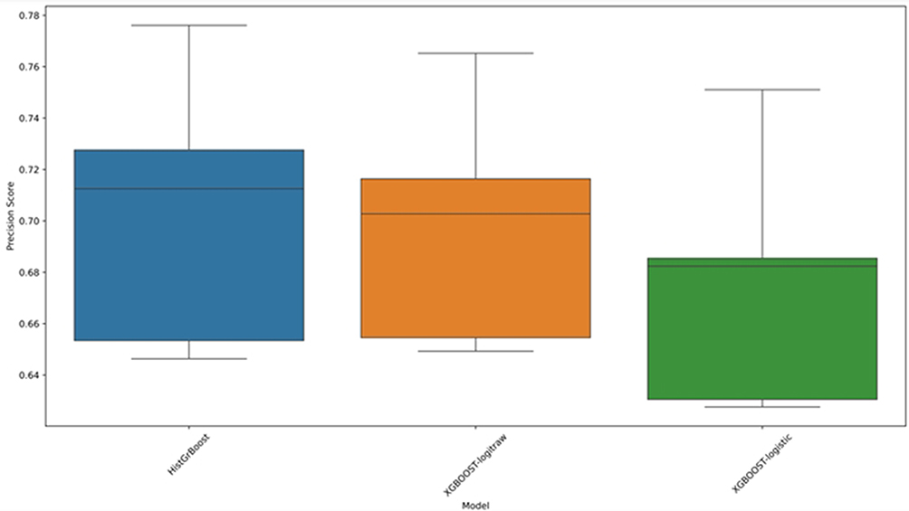Figure 11 Boxplot illustrating the precision scores of models capable of handling missing data.

As shown in Figure 11, HistGrBoost generally outperforms the XGBOOST variants. For additional validation of the performance of the models without excluding observations with missing values, we applied KNNimpute.³² Unlike simple imputation methods that use statistical metrics such as the mean, median, and mode, KNNimpute proved robust and provided an accurate estimation of the missing values according to.³² Table 7 illustrates the results of the models on the proposed dataset using the best-performing models (from the previous experiments) after applying the KNNimpute method.

Table 7 The Results of the Best Performers on the Proposed Dataset After Applying KNN Imputation. The Results Show the Mean ± Standard Deviation. Bolded Values are the Highest, for Each Metric

The results after performing imputation, to avoid excluding observations from the original dataset, show improvement in the performance of some of the models used. As shown in Table 7, compared to Tables 3 and 5, the SVM and LR evaluation metrics have slightly increased, in terms of precision and recall. However, the other models’ performances remain almost unchanged.

It is anticipated that employing the KNNimpute approach will result in an increase in performance, as shown in Table 7. This method works by determining the nearest neighbour instances for each case with missing data and then using these examples to impute the missing value using methods such as average, mode, or weighted average.

The p-values, Table 8, indicate a significant difference between SVM and both RF and HistGrBoost, suggesting that SVM performs differently from these methods. However, there is no statistical evidence to reject the null hypothesis when comparing RF with HistGrBoost, meaning their performance difference is not significant.

Table 8 The Bottom Triangle of the Table Shows the p-Values from the Wilcoxon Signed-Rank Test, Calculated for the Results in Table 8, Comparing the Performance of Each Pair of Classifiers. The Top Half of the Table Displays the Maximum Mean Precision for Each Classifier

Although this approach is more likely to be accurate and can improve decision boundaries and classification results, it cannot be guaranteed to be completely precise. Additionally, there are concerns about the reliability of synthetic data based on “more likely” estimates in medical decision-making. Recent research^33,34 suggests that synthesizing new data is a risky approach, especially in medical fields where misdiagnosis can have serious repercussions; therefore, other approaches such as ensemble learning or data partitioning³⁵ may be better alternatives.

The final set of experiments in this study is conducted using the best classifiers from the previous experiments. That is from the experiments of the clean data (without any missing values) we select RF and SVM and from the experiments on the dataset with missing values we select XGB1, XGB2 and HistGrBoost. In this experiment, we do not use the default parameters of the classifiers. Instead, we perform a grid search to find the best possible parameters that might increase the performance on the corresponding dataset. Table S2 shows each of these classifiers and their corresponding parameters that might impact the learning in each model. For more information about these parameters and their meaning, we refer the reader to SKlearn and XGBoost documentation pages.

After performing the grid search, we find the best parameters for each one of these classifiers as presented in Table 9.

Table 9 The Best Hyperparameter Values for Each Used Classifier

Table 10 and 11 show the results and the p-values, respectively, of SVM and RF classifiers trained on the clean version on the dataset using the parameters mentioned in Table 9.

Table 10 Results of SVM and RF Best Parameters Reported in Table 11. The Results Show the Mean ± Standard Deviation Over a 5-Fold Cross-Validation Test. Bolded Values are the Highest, for Each Metric

Table 11 The Bottom Triangle of the Table Shows the p-Values from the Wilcoxon Signed-Rank Test, Calculated for the Results in Table 12, Comparing the Performance of Each Pair of Classifiers. The Top Half of the Table Displays the Maximum Mean Precision for Each Classifier

Tables 12 and 13 show the results and the p-values, respectively, of XGb1, XGB2 and HistGrBoost classifiers trained on the dataset with missing values using the parameters mentioned in Table 9.

Table 12 Results of XGboost and HistGrBoost Best Parameters Reported in Table 11. The Results Show the Mean ± Standard Deviation Over a 5-Fold Cross-Validation Test. Bolded Values are the Highest, for Each Metric

Table 13 The Bottom Triangle of the Table Shows the p-Values from the Wilcoxon Signed-Rank Test, Calculated for the Results in Table 13, Comparing the Performance of Each Pair of Classifiers. The Top Half of the Table Displays the Maximum Mean Precision for Each Classifier

As one can observe from Table 10, Table 11, there is no significant difference of these optimized parameters from the default parameters. SVM and RF show high p-values, indicating that their performance is almost similar. However, Tables 12 and 13 show that optimized XGB1 and XGB2 are now performing better than the HistGrBoost according to their corresponding p-values, which provide a strong evidence to reject the null hypotheses. While the performance of XGB1 and XGB2 is almost similar without any significant difference.

It is important to note that examining the performance of models on such datasets is not only intriguing but also yields significant opportunities for further research, each of which could be a study in its own right. However, in our experimental study, we outline potential research paths that future researchers might consider exploring. This approach not only showcases our contributions but also sets the stage for ongoing inquiry and development in the field.

Discussion

This work demonstrated the feasibility of predicting cancer by analysing the components of CBC using a predictive modelling method. To maintain objectivity and prevent bias, we implemented a study design involving anonymization of patient. Initially, we built and trained the predictive model using an array of derived data. One of the datasets contained information about individuals who had been diagnosed with cancer; the second included non-cancer patients who had various chronic diseases that impacted the results of their CBC. Future prospective clinical research could offer a more precise assessment of the effectiveness of our methodology. The employed modelling approaches accurately distinguish between patients with malignant and benign conditions. The CBC findings were acquired from medical records collected from multiple hospitals in Jordan. As a result, the proposed method offers a wider range of population coverage and is more generalizable.

We demonstrated the utility of CBC data in providing vital insights into the presence of malignancy and its significance in clinical prediction models. In comparison, symptom-based models are limited by their inherent nature, as symptoms may not manifest until later stages of the disease. Moreover, individuals have the option to disregard or withhold information about their symptoms.²

Initially, we used RF feature priority ranking to highlight important features more efficiently. In this respect, “more efficiently” refers largely to the RF model’s capacity to rank features according to their relevance scores, allowing us to find the most significant factors for predicting outcomes without requiring considerable manual selection. This method not only speeds up the feature selection process but it also improves the accuracy of our model by focusing on the most useful features. Since the dataset contains several CBC test results for each patient, it was possible to include every statistical feature for every CBC parameters (for instance, the mean, standard deviation, and median), which resulted in the identification of the 60 most important features. Including different blood parameters, both as a multiple measurement and as a change over time, increased the model’s prediction power and might show a longer-term shift in blood parameters rather than a transient one.

In this work, we only used the RF model for feature selection, which may have introduced biases inherent in a single model’s perspective. However, we used 5-fold cross-validation during the model training process, which helps to reduce biases and offers a more trustworthy assessment of the model’s performance.¹⁵ Using a variety of models, such as an ensemble method with stacking feature importance, might improve feature selection robustness and generalization.³⁶ This restriction is significant since it may impact the reproducibility and reliability of our findings. As a result, it is critical that we assess and contrast the advantages of ensemble feature selection approaches in our future work.

We constructed a computational model utilizing an extensive dataset consisting of cancer and non-cancerous observations. Our methodology utilizes innovative techniques in feature selection, employing z score normalization to standardize feature scales. Additionally, we employ both linear and nonlinear modelling approaches to effectively manage sparse and chaotic information across time.

Choosing the optimal ML model requires meticulous examination. We assess the efficacy of a composite of classifiers, including RF, ANN, KNN, XGBOOST, AdaBoost, SVM, CTELC, and EE, on the provided dataset. Our results demonstrated that the RF model exhibited superior performance compared to the other models in accurately identifying cancer patients. This discovery illustrates the significant improvement that our model provides compared to current knowledge.¹⁴ The RF, SVM and LDA models demonstrated greater performance on the dataset of Jordanian patients, further substantiating their superiority, the RF model achieved an accuracy of 0.704 ± 0.044, the SVM model reached an accuracy of 0.705 ± 0.040, and the LDA model demonstrated an accuracy of 0.699 ± 0.049. In comparison, other models performed similar to LDA or even lower than 69.9% of accuracy. Tree-based models outweigh all other models (SVM, NN) in our study as well as in other studies.¹⁶

We have demonstrated that our approach outperforms other investigations that rely on a single or limited number of blood components for making predictions (e.g.,³⁷). This is accomplished by utilizing the full parameters of the CBC, trends in their values, sex, and age.

Based on the RF feature importance ranking, the WBC counts were determined to have the greatest impact. Moreover, the platelet count, age, and red blood cell count are notable attributes. Radiation therapy and chemotherapy can lead to a decrease in white blood cell count, as the bone marrow has decreased activity in patients who have been diagnosed. During the early diagnostic stage, the WBC count can serve as a reliable indicator of systemic inflammation, which has been associated with increased cancer risk and mortality rates in many studies. An association between WBCs and the risk of developing cancer has been documented in both lung cancer³⁸ and breast cancer^39. An observational study in the United Kingdom examined the association between WBC ratios and a heightened risk of cancer and mortality.⁴⁰ The study demonstrated a greater occurrence of colorectal and lung cancer risk as the number of cells increased. It has also been proposed that the WBC count and WBC ratio might be used as biomarkers to predict the risk of developing cancer, allowing for early detection of the disease up to one year before clinical diagnosis.

RBC count is a significant CBC result. RBC count is correlated with several CBC parameters, including haematocrit, MCV, MCH, MCHC, and RDW. Several studies have detailed the connections between cancer and these parameters. Moreover, the RBC counts MCV and MCH have been used in ML predictive models in the context of CRC.⁴¹ The model obtains between 98 and 99% accuracy when applied to data from different populations.¹⁶

The correlation between platelet count and cancer incidence is significant since it serves as an indicator of hemostasis in clinical settings. An increased platelet count has proven to be a useful indicator of cancer¹¹ and a risk factor for cancer.⁴² Furthermore, investigations examining the relationship between platelet count and survival in individuals recently diagnosed with cancer have revealed that many patients exhibit thrombocytosis (defined as a platelet count exceeding 450,000/μL).⁴³

Patient age was a strong indicator of the presence of cancer in our predictive model. The significance of age suggests that cancer continues to impact individuals who are already susceptible, specifically older people with many health conditions, particularly those with compromised physical and mental well-being who are prone to illness. The National Cancer Institute (NCI) states that advancing age is the primary risk factor for cancer in general and for many specific forms of cancer.⁴⁴ Some researchers have linked this trend to a decrease in immune system activity⁴⁵ and a deterioration of cellular function.⁴⁶ Research conducted on the Jordanian population indicates that age has a fluctuating impact on the occurrence of cancer.³

Similar to past studies in this field, our research is subject to specific constraints. While CBC data are readily available in Jordan, creating accurate forecasts using these data is notoriously difficult due to uneven testing or inadequate data collection. One further limitation of our study is that we verified our findings by retrospective analysis. However, we have presented a prediction equation that is mathematically bound to align with the principles of biology and medicine for any possible CBC test. As mentioned in the methodological description, we chose not to calibrate the model and instead utilized its free parameters. This approach enables us to determine the most suitable ML models with greater accuracy.

The current model exhibits good performance when evaluating unseen data by employing 5-fold cross-validation, ensuring both training and testing of all the data. However, the maximum diagnostic accuracy reached is merely 72%, which may be satisfactory for certain applications but falls short for medical purposes. In comparison to those of medical doctors, our outcomes might seem inadequate. This disparity arises because our model solely depends on blood tests and demographic factors such as age and sex, whereas medical professionals utilize extra information such as tumor markers, imaging, and scans to enhance their diagnoses. By integrating these additional data into the ML model, we could significantly boost its diagnostic accuracy since more comprehensive data would enable it to make more precise decisions. Such improvements can be made in our future work.

Conclusion and Future Work

We have introduced a predictive modelling approach to enhance the detection of cancer by evaluating age, sex, and comprehensive CBC information, which is often available in the electronic medical records of Jordanian hospitals. Our research focused on analysing the frequency and features of cancer in Jordanian patients. Additionally, we examine the pros and drawbacks of several predictive modelling methods in this specific context.

In future studies, there is a vast potential to expand upon the predictive modelling techniques used in this research by incorporating advanced methodologies. Exploring deep learning methods could provide insights into more complex patterns within the dataset, potentially improving the accuracy and robustness of the predictions.^47–50

Another avenue for enhancement involves experimenting with different imputation techniques to manage missing values in the dataset. Current methods, while effective, have limitations that novel imputation strategies could overcome, thereby refining the overall quality of the dataset and the resultant model performance.

Furthermore, broadening the focus of our study to encompass multiclass categorization would provide a more thorough evaluation of machine learning’s capacity to forecast different kinds of cancer. The use of numerous tumor markers in addition to blood tests and further investigation of their relationship are made possible by the multiclass classification approach. This extension would offer a more comprehensive comprehension of the models’ possible applications across various cancer classifications.

In addition to other methods, hyperparameter tuning for models such as support vector machines (SVMs) and random forests (RFs) represents a crucial area for future research. By optimizing these parameters, the predictive accuracy and efficiency of the models can be significantly enhanced, leading to more reliable and actionable results. It is important to highlight the need for further research to verify our results with larger and more varied datasets, since the incorporation of diverse datasets would allow for a more comprehensive validation of the models and their performance across different populations. Also, more advanced feature engineering methods like the interaction between features can be used in future research on this topic as it might increase the performance of the system. The comprehensive exploration of these advanced methods and enhancements cannot be adequately addressed within the confines of a single study. Each of these areas represents a substantial endeavour that could, individually, constitute a focused research project. Thus, our study lays the groundwork for these future explorations, which are essential for advancing the field of predictive modelling in medical diagnostics.

References

1. Cancer. 7, 2024. Available from:https://www.who.int/news-room/fact-sheets/detail/cancer.
2. Chapman BP, Lin F, Roy S, Benedict RHB, Lyness JM. Health risk prediction models incorporating personality data: motivation, challenges, and illustration. Personal Disord. 2019;10(1):46–58. doi:10.1037/per0000300
3. Ministry of health non-communicable diseases directorate Cancer Prevention Department (CPD) Jordan Cancer Registry (JCR) Email: [email protected].
4. Paquin AR, Oyogoa E, McMurry HS, Kartika T, West M, Shatzel JJ. The diagnosis and management of suspected lymphoma in general practice. Eur J Haematol. 2023;110(1):3–13. doi:10.1111/ejh.13863
5. Stauder R, Valent P, Theurl I. Anemia at older age: etiologies, clinical implications, and management. Blood. 2018;131(5):505–514. doi:10.1182/blood-2017-07-746446
6. Bosch FTM, Mulder FI, Huisman MV, et al. Risk factors for gastrointestinal bleeding in patients with gastrointestinal cancer using edoxaban. J Thromb Haemost. 2021;19(12):3008–3017. doi:10.1111/jth.15516
7. Divsalar B, Heydari P, Habibollah G, Tamaddon G. Hematological parameters changes in patients with breast cancer. Clin Lab. 2021;67(8). doi:10.7754/Clin.Lab.2020.201103
8. Spell DW, Jones DV, Harper WF, David Bessman J. The value of a complete blood count in predicting cancer of the colon. Cancer Detect Prev. 2004;28(1):37–42. doi:10.1016/j.cdp.2003.10.002
9. Hornbrook MC, Goshen R, Choman E, et al. Early colorectal cancer detected by machine learning model using gender, age, and complete blood count data. Dig Dis Sci. 2017;62(10):2719–2727. doi:10.1007/s10620-017-4722-8
10. Zhang P, Zong Y, Liu M, Tai Y, Cao Y, Hu C. Prediction of outcome in breast cancer patients using test parameters from complete blood count. Mol Clin Oncol. 2016;4(6):918–924. doi:10.3892/mco.2016.827
11. Giannakeas V, Kotsopoulos J, Cheung MC, et al. Analysis of platelet count and new cancer diagnosis over a 10-year period. JAMA Netw Open. 2022;5(1):e2141633. doi:10.1001/jamanetworkopen.2021.41633
12. Záhorec R, Marek V, Waczulíková I, et al. Predictive model using hemoglobin, albumin, fibrinogen, and neutrophil-to-lymphocyte ratio to distinguish patients with colorectal cancer from those with benign adenoma. | Neoplasma | EBSCOhost. 2021;68(6). doi:10.4149/neo_2021_210331N435
13. Chen X, Gole J, Gore A, et al. Non-invasive early detection of cancer four years before conventional diagnosis using a blood test. Nat Commun. 2020;11(1):3475. doi:10.1038/s41467-020-17316-z
14. Bandyopadhyay A, Albashayreh A, Zeinali N, Fan W, Gilbertson-White S. Using real-world electronic health record data to predict the development of 12 cancer-related symptoms in the context of multimorbidity. JAMIA Open. 2024;7(3):ooae082. doi:10.1093/jamiaopen/ooae082
15. Al-Khlifeh EM, Alkhazi IS, Alrowaily MA, et al. Extended spectrum beta-lactamase bacteria and multidrug resistance in Jordan are predicted using a new machine-learning system. IDR. 2024;17:3225–3240. doi:10.2147/IDR.S469877
16. Kinar Y, Kalkstein N, Akiva P, et al. Development and validation of a predictive model for detection of colorectal cancer in primary care by analysis of complete blood counts: a binational retrospective study. J Am Med Inf Assoc. 2016;23(5):879–890. doi:10.1093/jamia/ocv195
17. Li H, Lin J, Xiao Y, et al. Colorectal cancer detected by machine learning models using conventional laboratory test data. Technol Cancer Res Treat. 2021;20:15330338211058352. doi:10.1177/15330338211058352
18. Tsai IJ, Shen WC, Lee CL, Wang HD, Lin CY. Machine learning in prediction of bladder cancer on clinical laboratory data. Diagnostics. 2022;12(1):203. doi:10.3390/diagnostics12010203
19. Jia Y, Liu Z, Guo J, et al. Machine learning and bioinformatics analysis for laboratory data in pan-cancers detection. Adv Intell Sys. 2023;5(12):2300283. doi:10.1002/aisy.202300283
20. Kumar R, Saha P. A review on artificial intelligence and machine learning to improve cancer management and drug discovery. Int J Res Applied Sci Bio. 2022;9(3):149–156. doi:10.31033/ijrasb.9.3.26
21. Pant A, Sharma G, Saini S, et al. Quality by design-steered development and validation of analytical and bioanalytical methods for raloxifene: application of monte carlo simulations and variance inflation factor. Biomed Chromatogr. 2023;37(8):e5641. doi:10.1002/bmc.5641
22. Krouwer JS. Setting performance goals and evaluating total analytical error for diagnostic assays. Clin Chem. 2002;48(6):919–927. doi:10.1093/clinchem/48.6.919
23. Tarawneh AS, Alamri ES, Al-Saedi NN, Alauthman M, Hassanat AB. C℡C: a constant-time ensemble learning classifier based on KNN for big data. IEEE Access. 2023;11:89791–89802. doi:10.1109/ACCESS.2023.3307512
24. Liu XY, Wu J, Zhou ZH. Exploratory Undersampling for class-imbalance learning. IEEE Trans Syst Man Cybern. 2009;39(2):539–550. doi:10.1109/TSMCB.2008.2007853
25. Al-khlifeh EM, Hassanat AB. Predicting the distribution patterns of antibiotic-resistant microorganisms in the context of Jordanian cases using machine learning techniques. J Appl Pharm Sci. 2024;14(6):174–183. doi:10.7324/JAPS.2024.177584
26. Habbash M, Mnasri S, Alghamdi M, et al. Recognition of Arabic accents from English spoken speech using deep learning approach. IEEE Access. 2024;12:37219–37230. doi:10.1109/ACCESS.2024.3374768
27. Alkhawaldeh I, Al-Jafari M, Abdelgalil M, Tarawneh A, Hassanat A. A machine learning approach for predicting bone metastases and its three-month prognostic risk factors in hepatocellular carcinoma patients using SEER data. Ann Oncol. 2023;34:140. doi:10.1016/j.annonc.2023.04.414
28. Abujaber AA, Alkhawaldeh IM, Imam Y, et al. Predicting 90-day prognosis for patients with stroke: a machine learning approach. Front Neurol. 2023;14:1270767. doi:10.3389/fneur.2023.1270767
29. Molnar C. Interpretable Machine Learning. Lulu.com; 2020.
30. Ke G, Meng Q, Finley T, et al. LightGBM: a highly efficient gradient boosting decision tree. Adv Neural Inf Process Syst. 2017;30.
31. Guryanov A, et al. Histogram-based algorithm for building gradient boosting ensembles of piecewise linear decision trees. Analysis Images Soc Netwo Texts. 2019:39–50. doi:10.1007/978-3-030-37334-4_4.
32. Troyanskaya O, Cantor M, Sherlock G, et al. Missing value estimation methods for DNA microarrays. Bioinformatics. 2001;17(6):520–525. doi:10.1093/bioinformatics/17.6.520
33. Tarawneh AS, Hassanat AB, Altarawneh GA, Almuhaimeed A. Stop oversampling for class imbalance learning: a review. IEEE Access. 2022;10:47643–47660. doi:10.1109/ACCESS.2022.3169512
34. Hassanat A, Altarawneh G, Alkhawaldeh IM, et al. The jeopardy of learning from over-sampled class-imbalanced medical datasets. 2023 IEEE Symp Comput Commun. 2023:1–7. doi:10.1109/ISCC58397.2023.10218211.
35. Hassanat AB, Tarawneh AS, Abed SS, Altarawneh GA, Alrashidi M, Alghamdi M. RDPVR: Random Data Partitioning with Voting Rule for machine learning from class-imbalanced datasets. Electronics. 2022;11(2):228. doi:10.3390/electronics11020228
36. Teo PT, Rogacki K, Gopalakrishnan M, et al. Determining risk and predictors of head and neck cancer treatment-related lymphedema: a clinicopathologic and dosimetric data mining approach using interpretable machine learning and ensemble feature selection. Clin Transl Radiat Oncol. 2024;46:100747. doi:10.1016/j.ctro.2024.100747
37. Coradduzza D, Medici S, Chessa C, et al. Assessing the predictive power of the hemoglobin/red cell distribution width ratio in cancer: a systematic review and future directions. Medicina. 2023;59(12):2124. doi:10.3390/medicina59122124
38. Wong JYY, Bassig BA, Loftfield E, et al. White blood cell count and risk of incident lung cancer in the UK Biobank. JNCI Cancer Spectr. 2019;4(2):pkz102. doi:10.1093/jncics/pkz102
39. Park B, Lee HS, Lee JW, Park S. Association of white blood cell count with breast cancer burden varies according to menopausal status, body mass index, and hormone receptor status: a case-control study. Sci Rep. 2019;9(1):5762. doi:10.1038/s41598-019-42234-6
40. Nøst TH, Alcala K, Urbarova I, et al. Systemic inflammation markers and cancer incidence in the UK Biobank. Eur J Epidemiol. 2021;36(8):841–848. doi:10.1007/s10654-021-00752-6
41. Hilsden RJ, Heitman SJ, Mizrahi B, Narod SA, Goshen R. Prediction of findings at screening colonoscopy using a machine learning algorithm based on complete blood counts (ColonFlag). PLoS One. 2018;13(11):e0207848. doi:10.1371/journal.pone.0207848
42. Ankus E, Price SJ, Ukoumunne OC, Hamilton W, Bailey SER. Cancer incidence in patients with a high normal platelet count: a cohort study using primary care data. Fam Pract. 2018;35(6):671–675. doi:10.1093/fampra/cmy018
43. Ishizuka M, Nagata H, Takagi K, Iwasaki Y, Kubota K. Preoperative thrombocytosis is associated with survival after surgery for colorectal cancer. J Surg Oncol. 2012;106(7):887–891. doi:10.1002/jso.23163
44. Risk Factors: age - NCI. Available from: Available from: https://www.cancer.gov/about-cancer/causes-prevention/risk/age.
45. Hong H, Wang Q, Li J, Liu H, Meng X, Aging ZH. Cancer and Immunity. J Cancer. 2019;10(13):3021–3027. doi:10.7150/jca.30723
46. Pence BD, Yarbro JR. Aging impairs mitochondrial respiratory capacity in classical monocytes. Exp Gerontol. 2018;108:112–117. doi:10.1016/j.exger.2018.04.008
47. Tarawneh AS, Celik C, Hassanat AB, Chetverikov D. Detailed investigation of deep features with sparse representation and dimensionality reduction in CBIR: a comparative study. Intell Data Anal. 2020;24(1):47–68. doi:10.3233/IDA-184411
48. Hassanat ABA, Albustanji AA, Tarawneh AS, et al. DeepVeil: deep learning for identification of face, gender, expression recognition under veiled conditions. Int J Biomet. 2022;14(3–4):453–480. doi:10.1504/IJBM.2022.124683
49. Tarawneh AS, Hassanat AB, Alkafaween E, et al. DeepKnuckle: deep learning for finger knuckle print recognition. Electronics. 2022;11(4):513. doi:10.3390/electronics11040513
50. Fararjeh AF, Alkhlifeh E, Aloliqi A, Tarawneh A, Hassanat A. The use of gene expression profiling to predict molecular subtypes of breast cancer by a new machine learning algorithm: random forest. Curr Bioinf. 2024;20. doi:10.2174/0115748936314079240827062219
© 2025 The Author(s). This work is published and licensed by Dove Medical Press Limited. The
full terms of this license are available at https://www.dovepress.com/terms.php
and incorporate the Creative Commons Attribution
- Non Commercial (unported, 3.0) License.
By accessing the work you hereby accept the Terms. Non-commercial uses of the work are permitted
without any further permission from Dove Medical Press Limited, provided the work is properly
attributed. For permission for commercial use of this work, please see paragraphs 4.2 and 5 of our Terms.