Sex-Specific Ensemble Models for Type 2 Diabetes Classification in the Mexican Population

Introduction

Type 2 Diabetes (T2D) is an ailment in which 2 conditions occur in the body: Insulin resistance and/or insulin deficiency (either lack of insulin production or ineffective insulin production).¹ The American Diabetes Association (ADA) ² mentions that most of the effects go unnoticed until they are already advanced. T2D is acquired through poor eating habits, lack of exercise and even heredity,³ however, it is preventable. An early diagnosis helps to prevent the affectations that may be acquired over time, and this becomes a challenge because the symptoms are usually silent and when they appear diabetes is already advanced.

According to WHO,³ 422 million people worldwide have diabetes and 1.5 million deaths attributed to diabetes each year and increasing. In Mexico, according to Basto-Abreu et al⁴ in an article published in the Mexican Journal of Public Health, there are about 14.6 million Mexicans, representing 18% of the population, with this condition and female having the highest incidence with 52.4%, being the 20.1% diagnosed with diabetes and 32.3% undiagnosed. And it is estimated that a high percentage of the population remains undiagnosed.⁴ Therefore, it is essential to develop tools that facilitate the early diagnosis of these conditions, considering males and females separately due to their biological differences.⁵ This is why it is essential to develop inexpensive tools that can support the early diagnosis of these conditions by reducing the number of characteristics to be analyzed, given the medical urgency and the large number of people at risk. These tools should also account for males and females separately due to the biological differences between them.

While machine learning (ML) has been widely applied to type 2 diabetes classification, most studies treat the population as homogeneous and do not consider sex-specific differences in clinical or metabolic characteristics.^6–8 This limits the potential of these models to support more accurate and equitable diagnoses. Considering the known biological differences between males and females, there is a growing need for ML approaches that account for sex-based variability. Ensemble learning methods, which integrate the predictions of multiple algorithms, have demonstrated strong performance in biomedical research and clinical prediction tasks.^9–12 They have also been successfully applied in the prediction of diabetes. For example, Binte Kibria et al¹³ developed an interpretable ensemble-based model using SHAP values to explain predictions and increase clinical trust. Similarly, Singh et al¹⁴ proposed eDiaPredict, a hybrid ensemble model for diabetes classification that achieved 95% accuracy. While technically strong, these models do not consider sex-specific variability, further reinforcing the need for personalized ensemble approaches tailored to diverse populations. Their flexibility and robustness make ensemble models promising tools for building sex-specific diagnostic systems, although their use in this context—particularly in underrepresented populations such as the Mexican demographic—remains limited.

On the other hand, personalized medicine¹⁵ is an emerging science that relies on the genetic profiles of individuals to guide from diagnosis to better treatment. As the National Human Genome Research Institute says, it is an opportunity to change that “It’s a one-size-fits-all” approach, talking about diagnosis and treatments. There is no doubt all people are very similar, and at the same time the differences are notorious. The genomics level is opening the doors to make these differences more visible,¹⁵ making it so that when dealing with the patient to give those diagnoses, treatments, medication, etc. based on the differences to reach these potential milestones in medicine.

Therefore, the present study aims to take advantage of the robustness of ensemble models and feature selection to apply personalized medicine based on sex, considering the high genetic variability in the Mexican population, and to improve diagnostic accuracy and patient care by reducing the number of characteristics to be analyzed.

Materials and Methods

This section describes data analysis for the creation of classification methods and presents four main phases: data splitting, feature extraction, validation and performance testing.

Generally, the process began with acquisition of the data set (DS), followed by statistical analysis of the data, and then cleaning, which consists of removal of “N/A” and unique features such as diabetes treatments, and finally separation of the data by sex (female and male).

The subsets of data by sex are separated into 80% for training and feature extraction, and the remainder is used for blind testing. Then, from each subset of data, feature selection is performed using GALGO, Genetic Algorithms to solve Optimization. The effectiveness of these features from each subset is then evaluated using classification techniques: Random Forest (RF), K-Nearest Neighbors (KNN), Logistic Regression (LR), and Support Vector Machines (SVM). Subsequently, the models are evaluated to find the best performance. The methodology ends with the assembly of the models evaluated by sex, evaluating the performance in the early detection of T2D according to sex with the blind test. Figure 1 presents a summary for the data management process to go through the process of analysis, model creation and classification.

Figure 1 Model ensemble training methodology summary. Figure shows a flow chart where a dataset statistical analysis is performed. The data is then cleaned to be used by the AI tools. After the analysis and cleaning data process, the rest of flowchart it is made twice, one for female dataset and one for male dataset in order to get two final ensemble models.

Data Processing

Dataset Description

The DS was provided by the “Instituto Mexicano del Seguro Social Hospital Siglo XXI” in Mexico City, MX. The DS was previously approved by the hospital’s ethics committee under approval R-2011-785-018. It consists of a total of 1787 instances, with 895 female and 892 male cases. Additionally, the DS includes 34 features, along with case and control labels. These features encompass sociodemographic, clinical dichotomous, and other relevant variables.

Data Preprocessing

The preprocessing of the DS is performed in RStudio (4.1.3) with the help of dplyr.^16,17 This DS is made up of 34 characteristics, some of which are defining characteristics of diabetic patients, such as treatment for diabetes, age at diagnosis, among others, which if used during the selection phase of the characteristics would be highly significant for their classification, since non-diabetic patients would not have treatment or age at diagnosis. Thus, they are eliminated because they are features that occur after diagnosis and are specific to the case group. Similarly, non-relevant or random features, such as Patient ID, are removed as they may interfere with the training stage of the model. The work of the algorithms is based on decision rules based on the mathematical relationship of the features. When any space is null or empty it is called N/A, making it impossible to establish this relationship. This process directly interferes with algorithm training and modeling. As a next step, a search for missing values (N/As) in the DS is conducted, and rows with missing data are eliminated to avoid artificial data imputation. This decision aligns with the principles of genetic algorithms and nature inspired models, which aim to preserve the natural integrity of the data. The remaining data are summarized in Table 1. Tables 2 and 3 present a frequency on factor features for female and male, respectively, Tables 4 and 5 describe statistically the metrics on female and male populations.

Table 1 Postprocessed Data Remaining Features

Table 2 Counts on Female Factor Features

Table 3 Counts on Male Factor Features

Table 4 Statistical Description on Female Numeric Features

Table 5 Statistical Description on Male Numeric Features

Data Division

It is well known that there are physiological, anatomical and pathological differences, among other branches of health sciences⁵ between male and female population, according to this, the DS division is made with the intention of finding if there is a difference between risk characteristics between male and female, and if so, to what risk factor they are given. Chowen et al¹⁸ point out that male and female respond differently to the various metabolic challenges they face. The hypothalamus is the central part of metabolic control and that the cycles it manages are based on the sex of the patient and respond differently to metabolic signals. In the same way, it says that the accumulation of body fat in female is important for reproduction and care of offspring. Complementing this, Szdavari et al¹⁹ states that female and male differ in combinations of hormonal and genetic factors such as sex hormones, environmental factors where they develop among others. Based on previous research by other authors, it is decided to divide the DS by sex and to search for the varied factors that may exist between male and female.

After that, the division of the data is given in 80% for training and 20% for testing, this in order to have a training set and a blind set. This is done to train the model with the training set, obtain performance measurements and with this to test and validate its reliability with the blind set. The resulting DS division is summarized in Table 6.

Table 6 Partitioning of the Data Set for Training and Testing. Columns Represent the Resulting Data Sets (by Sex), and Rows Represent What They Will Consist of (By Case/Control)

Programming

The programming and everything described in this section is done with the R programming language in RStudio in 4.1.3 version with the following packages: pROC 1.18.0,²⁰ caret V6.0–94,²¹ corrplot V0.94,²² e1071 V1.7–13²³, dplyr V1.1.2^16,17 and GALGO V1.4²⁴ and Python.

Features Extraction

In this section, GALGO package in R is used as a feature extractor for the male and female databases. As described by its authors, “GALGO is a generic software package that uses Genetic Algorithms to solve Optimization problems involving the selection of variable subsets”.²⁴ It is implemented in the R programming environment, and utilizes the foundation of genetic algorithms, which mimic biological survival, where only the most relevant features “survive”. Genetic algorithms are procedures of searching for the best variables (these being equivalent to chromosomes) using the principle of natural selection, randomly combining the population, cycling, recombining and mutating the chromosomes that best fit. All this with the advantage of analyzing large amounts of data in an optimal and fast way without neglecting the high fit values and implementation functions for the analysis of the same. A brief description of how these models (chromosomes) are managed is presented in Figure 2.

Figure 2 Schematic representation of the Genetics Algorithms Procedure. Specifically on step 3, the algorithm iterates until the fitness equals or gets above our goal.

To ensure stable characteristic extraction using genetic algorithms, it is crucial to carefully define the number of solutions. Several studies^9,25–28 recommend setting this number to at least twice the greater value between the number of characteristics and the number of samples in the dataset. In this study, the dataset comprises 34 characteristics and a total of 1202 patients, 633 males and 569 females, so the number of solutions is determined based on the sample size. Accordingly, the maximum number of generations (solutions) is set to 1200, allowing the algorithm sufficient iterations to explore the search space and converge toward optimal solutions.

The characteristic extraction process is configured with a chromosome length of 5 and a classification method based on the “near center” approach. Following the methodology proposed by Garcia-Hernandez et al²⁷ and Escobar et al,²⁹ a perfect fitness target of 1.0 is used to maximize accuracy and to ensure the selection of the most relevant and reliable combinations of characteristics.

In both the male and female datasets, 80% of the samples, originally allocated for training, are first used to perform the characteristic extraction. This ensures that feature selection is guided by the same data that will later be used to train the predictive models, maintaining consistency and reducing the risk of information leakage. The same procedures are applied independently to each group to enable fair comparison.

Cross-Validation

Cross Validation (CV) is one of the methods used to prevent overfitting of predictive models and when applying it with blind data it can be effective.³⁰ It is used to estimate the real error prediction in the models and adjust the parameters. The “k-fold cross-validation” method divides the training dataset into k-folds or subsets to make use of the training model with k-folds −1 known as training set and predicts the remaining k-fold called validation set, making a repetitive process until all the k-folds are predicted by the models trained with the other k-folds.

In this study, the splitting is done with k = 10. A graphical representation is presented in Figure 3. It is important to note that a CV must be performed individually for each model to be trained. This CV method is used to validate the input models that will be included in the ensemble model. This process is implemented on Python and R on caret package.

Figure 3 Cross-validation scheme. In each iteration the validation set goes on every fold of the CV, until every fold is a validation set at least once. The image shown an example in a k = 5 parameter.

Classification Models

Different sex-sorting algorithms are proposed, along with a comparison of their performance by sex using the features extracted by GALGO. The algorithms selected for this study are SVM, RF, LR and K-NN. The choice of these algorithms is based on their performance, frequency of use in related work, and computational efficiency.

SVM is a supervised algorithm that searches for the optimal hyperplane to separate the data and make the data selection.³¹ One of the main features of SVM is that it uses different types of hyperplane shapes based on different mathematical functions to separate the data in different ways. These functions are called Kernel and can be: Linear, polynomial, radial or sigmoid and these are part of some of the advantages of this algorithm. Another advantage is that it can work with many samples without much computational demand. As IBM explains it,³² the data will be mapped according to the characteristics of each observation as shown in the Figure 4a even without being linearly separable. When a separator is found between categories as shown in the Figure 4b, the data is transformed so that this separator can be a hyperplane shown in the Figure 4c. Subsequently, the algorithm creates margins known as support vectors, which are the limits between the categories, as in the Figure 5a to further improve the model’s accuracy. SVM looks for these support vectors to be as wide as possible as shown in the Figure 5b, as they will help us to make the model more accurate.

Figure 4 (a) Data mapping. (b) Generation of the data separator line between classes. (c) Transformation of the data.

Figure 5 (a) The supports are generated with a limit on the first observations found in any of the categories. (b) Optimization is performed until the supports are as large as possible.

RF is a supervised learning algorithm based on decision trees that consists of creating several decision trees from the training data^33,34 and combining the predictions that each tree gives individually. A decision tree is a supervised learning algorithm, which is used for classification or regression tasks. It has a “tree” structure, hence the name, consisting of a root, branches, internal nodes and leaves as shown in Figure 6.

Figure 6 Decision tree basic structure.

The outgoing branches from the node derive in leaves in case of having another characteristic they become internal nodes and from here there are more branches to give rise to even more leaves. The branches form homogeneous subsets based on the available features in a repetitive manner until a final decision leaf is reached. For binary classification with an output label 0 and 1, the real values of the linear regression model need to be converted into 0 and 1 establishing a threshold, which is a numeric value between 0 and 1 where lies the decision to get into 0 or 1 classification. For classification, we need a function where we can differentiate between 0 and 1, the most common is the logistic function shown in Equation 1.

(1)

Based on this, we can find the probability that a sample is classified in some portion of our function, and thus, with the threshold establish whether it belongs to a class 0 or 1.³⁵ The logistic regression is represented in Figure 7.

Figure 7 Logistic Regression and Logistic Function.

Figure 7 Logistic Regression and Logistic Function

KNN³⁶, it is a supervised sorting algorithm, using a method that identifies a group of k samples already mapped as can be seen in Figure 8a, the algorithm identifies the distances between the group and the unknown sample in order to assign them to the group. When an observation to be classified by the algorithm is mapped as the Figure 8b presents, it looks for the distance in relation to the others and thus to know its closest point,³⁷ by this comes the name of this algorithm. To know the distances, several methods are used where the Euclidean distance, showed on Figure 8c, that consists of a straight line to the reference point or neighbor and the Manhattan distance that creates straight lines both horizontally and vertically, adding these 2.

Figure 8 (a) Mapping of the data. (b) Integration of a new observation. (c) Measurement of distances and classification.

The hyperparameters of the algorithms are prepared according to their nature and are the same for each sex-specific model. The RF models are trained with 100 trees and with one seed to replicate training. The logistic regression only applied a seed hyperparameter and finally SVM, which is set to a Radial Basis Function kernel.

Ensemble Models

Ensemble learning, also known as multi-classifier learning, combines the outputs of multiple models to solve a problem. These models use the predictions generated by other models to produce a final output, which can be either binary or numerical. Ensemble learning involves creating a “stacking of multiple models” to complement each other, enhance robustness, and improve overall performance. Among the diverse types of ensemble models stand out by taking the probabilities provided by other models and using them as input features for final training. This approach further increases the robustness and accuracy of the model. A diagram illustrating this type of model is presented in Figure 9. Each sex-specific model had its own ensemble model, established with different models to converge to a metamodel, which will define the final classification of the entries. For the female sex model, the initial estimators are: RF, LR, and SVM, with an ensemble metamodel with SVM with RBF kernel. For the male model, only 2 initial estimators are used: RF and SVM with an ensemble metamodel of RF with 100 trees. The decision to use these input models and the final model is explained in more detail in the results section.

Figure 9 Summary diagram of a stacked ensemble model.

Performance Evaluation

To measure the performance of the models during CV and of the model with the training set to predict the blind set, common evaluation metrics such as accuracy, which indicates the number of samples correctly classified, sensitivity, which is the ability to correctly classify positive samples, and specificity, which indicates the ability to correctly classify negative samples, are also used. Metrics like the ROC (Receiver Operating Characteristics) curves are also used.³⁸ These are two-dimensional metrics for evaluating the performance of classification models by plotting the probability of hitting examples as true positives against the probability of hitting true negatives. From these ROC curves, it is possible to obtain metrics to evaluate the performance of the models in different domains such as specificity, this will tell us how good the model is at predicting true negatives. Sensitivity will help us to know how accurate the model is with those who are positive and accuracy as a global metric of how good it is to classify patients in its original status. Finally, one of the most commonly used is the AUC (Area Under the Curve) which will be generated from a graphic threshold of specificity and sensitivity together indicating how good it is overall. Adding another one metric, F1 Score, which offers a useful alternative to a simple misclassification rate using precision and recall.³⁹ The formulas for the calculation of these metrics are shown in equations 2, 3, 4, 5 and 6. The confusion matrices are also obtained by means of Corrplot and caret in RStudio.

(2)

Results

Statistical Analysis

To gain a clearer understanding of the dataset, a basic descriptive analysis is conducted. This includes the evaluation of quartile distribution, means, medians, and other statistical measures. Particular attention is given to characteristics such as age and glucose levels, as these are established biomarkers of type 2 diabetes. The analysis also emphasizes differences between female and male participants, as well as between case and control groups. Here are able to see that in the female’s DS the patient data is distributed between 30 and 84 years, although half of the data is between 47 and 60 years as indicated by the 1Q (First Quartile) and 3Q (Third Quartile). While in the male’s DS there is a range that goes from 30 to 86, and in this one, the data is more concentrated in the center since half of the patients are between 43 and 58 years old. To graphically show the above, the box plots are shown in Figure 10a.

Figure 10 (a) Boxplot of age divided into males and females. (b) Blood glucose levels divided into males and females. The colored box represents the IQR, and the middle bold line highlights the median (Q2). The lines on under and top are the whiskers (Q1 and Q3 respectively) Over the top of the whiskers, the outliers are represented by circles.

However, the boxplot diagrams show that in both male and female there are outliers that make sample range increase, and that in reality the sample distribution is between 30 and 80 for male and between 30 and 77, and that the mean for female is higher than for male.

Speaking about a second variable, blood glucose is one of the most widely used measures currently used for DT2 diagnosis. Figure 10b presents the box-and-whisker plots of these variables.

There are many outliers in this variable since its range in any sense is very wide and can be caused by a bad intake, not complying with the correct fasting, among other things.

However, in male, their normal distribution ranges from 38 to 538 mg/dl (milligrams per deciliter), and that for their IQR (Interquartile range), where half of their data is present, it is in a range of 81 to 113 mg/dl, which is very close to the measure established as safe by the WHO in fasting conditions. Looking at the boxplot of female, the situation changes because despite not having outliers as high as in the case of male, their sample distribution is in higher values ranging from 59 mg/dl to 428, and similarly both their IQR are still in high values compared to male presenting values of 87, 97.5 and 140 mg/dl in each quartile, respectively. Glucose is an important reference to describe diabetes. In female, it ranges from 59 to 428 mg/dl, and in male, it ranges from 81 to 538 mg/dl. Figure 11 presents how glucose is distributed according to the age of the patients.

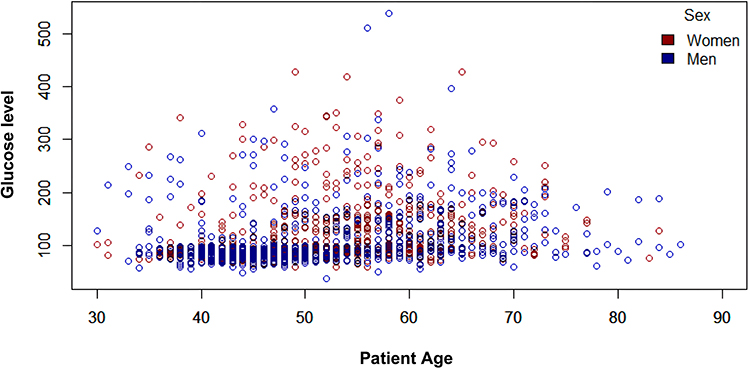Figure 11 Age distribution of patients with blood glucose level (mg/dl) divided by sex. Labeled as, red dots represent women instances, and blue represents men instances.

Based on the above able to conclude that female have higher distribution values despite their ages are not so different compared to those of male and it is important to mention that, as can be observed, the highest glucose levels are found between 50 and 70 years of age, regardless of sex.

Features Extraction

First, the training DS of each sex is entered in GALGO, to obtain separately the characteristics that could define each sex. Figure 12a presents the frequency of occurrence in the genes (variables) of the chromosomes (models) for the female population. It is observed that the genes with the highest frequency are “Age”, “Glu” and “Crea”, however, this is not the only thing to consider since some genes are always good, but there are also those that in combination with others do not have good yields for the chromosomes. Likewise, and under the same criteria, the frequencies and stability of the genes for the male population are shown in Figure 12b. Also, in Figure 13a presents the gene ranks plus the frequency where the continuity of the colors of each gene gives us the stability or performance accompanied by other genes. This Figure presents the Gene and frequency of the genes. As can be seen, “Age”, “Glu”, “CREA”, “HDLc” and “DBP” have a high frequency and stability, concluding these are the features with the highest predictive capacity in the DS.

Figure 12 (a) Frequency of the presence of each “gene” (variable) in female (b) Frequency of the presence of each “gene” (variable) in male.

Figure 13 (a) Stability of each “gene” in female (b) Stability of each “gene” in male.

In Figure 13b is visible, the genes change in ranking, removing the “CREA” for males and showing the “UREA”. It is also observed that in males, there are only 4 genes that are significant under these parameters, while in females 5 are presented, significantly reducing the number of characteristics needed to perform quality classifications compared to other related work presented below in the discussion section.

Even so, it is important to continue investigating the results, so the following are the processes of Forward Selection Models for both populations. GALGO also gives us the opportunity to extract the best model from the forward selection model technique. Figure 14 presents highlighted as a black line, which model is recommended to use and the number of features for the model to be effective.

Figure 14 (a) Forward Selection models given by GALGO in female population (b) Forward selection models given by GALGO in male population.

Figure 15 ROC curve for the models to be used in females metamodel.

As the figures show in both cases, the dotted black line presents the model’s ability to correctly predict the cases, the red line indicates the predictive ability for the controls and a bold black line the overall performance of the model. On the left side, a black line stands out, which indicates the model that GALGO recommends being used, showing in the lower X axis the features to be used and in the upper X axis the number of features that the model would have. In Figure 14a it is recommended the use of the model number 2 for female and in Figure 14b the model number 1.

Despite having a reduced number of variables, it is opted for the use of Robust Backward Gene Elimination (RBGE), which reduces the number of traits to the truly significant ones. Figure 14 presents the features of the models. In female, they are initially “Age”, “GLU”, “CREA”, “HDLc”, “DBP”, “BMI” and “UREA” and after the RBGE the variables “CREA” and “UREA” are eliminated giving 5 initial features for female models. In the case of male, the initial variables are “Age”, “GLU”, “DBP”, “UREA”, “HDLc” and “Edu” and after RBGE it reduced us to “Age”, “GLU”, “DBP”, “HDLc” and “Edu”. These final features are used to train the classification models, giving 5 features for each model.

Classification Models

For the model training process, four classification models are trained with the different methods presented above. The confusion matrices obtained from each classification model for female are presented below.

Classification Models for Female Population

For each classification model, 10-k folds are used for the CV process. The confusion matrices obtained for each model on prediction for the blind set are shown in Table 7.

Table 7 Confusion Matrix for Female Population on Blind Set

And the performance measures for each model are shown below in Table 8.

Table 8 Performance Measures on Blind Set in Female Population by Model

Looking at the confusion matrices and performance measures, it could choose the ones with the best performance for the creation of the ensemble model; however, the ensemble models are to create a robustness to the model that, generally combining performance, also combines the classification methods. Combinations are made between several models and finally the best performances are found with the RF, LR and SVM models for the female model. As can be seen, all models perform efficiently, with results above 88% in their main metrics. Likewise, combinations made in the model assembly of each one of these, discarding each one until the ideal combination with the best results is found, which in the case of female is a combination of RF, LR and SVM.

Figure 15 presents how the models behave on a ROC curve, and the same Figure presents the AUC value, these models are trained with the training set and predicting the blind set.

Classification Models for Male Population

The same CV parameters are used as in the results for the female’s population, 10-k folds. The confusion matrices obtained for each model in male population are shown in Table 9.

Table 9 Confusion Matrix for Male Population on Blind Set

And the performance measure for each model is shown in Table 10 below.

Table 10 Performance Measures on Blind Set in Male Population by Model

Males take higher values than female, denoting an ease in the classification of the male’s population. In the case of male, the metrics are higher, being higher than 93% in each of them. As mentioned above, different combinations are made with the proposed models, being finally selected 3: RF, KNN and SVM as the predecessors to create the ensemble model.

Figure 16 ROC curve for the models to be used in male presents how the models behave on an ROC curve and gives an approximation of the behavior of the model ensemble, which will be shown below. These models are trained with the training set, and the resulting model is used to predict the blind set.

Figure 16 ROC curve for the models to be used in male metamodel.

Stack Ensemble Models

As shown above, stacked ensemble models help us combine model predictions to obtain greater certainty and robustness in the classification using as input the classification probability calculated by the models, this probability is shown as OFF, Out of The Fold. The OFF values are obtained for each of the models in the train data, to know the probabilities calculated during the CV process and being added to the DS. Likewise, the OOF values are obtained for the blind data to create a confusion matrix for the ensemble model. As mentioned above, the RF and KNN models are selected as predecessors and SVM as the ensemble model for female and RF, KNN and SVM for male serving as input to the SAM, Stacked Assembly Model. Table 11 Best models sum and each metamodel metrics for female presents the performance metrics of different model combinations and metamodels in a classification task, comparing accuracy, specificity, sensitivity and F1 score. The model combination of RF + LR + SVM using as SVM metamodel achieves the highest overall performance. This indicates that this model is highly accurate in its predictions, particularly effective in correctly identifying negative cases, while maintaining a strong balance between accuracy and recall. In contrast, the model with LR metamodel demonstrates the best sensitivity, making it the most accurate in identifying true positives.

Table 11 Best Models Sum and Each Metamodel Metrics for Female Population

Table 12 Best models sum and each metamodel metrics for male showcases the performance of diverse model combinations and metamodels. The RF + SVM model with a RF metamodel presents the best accuracy (92.45%) and sensitivity (89.09%), making it the most balanced model for correctly identifying both true positives and true negatives. The RF + KNN model with SVM metamodel exhibits the highest specificity (97.11%). Whereas the RF + LR with KNN metamodel has the lowest accuracy and F1 score, indicating less effective overall performance, particularly in balancing accuracy and recall. Finally, the RF + KNN model with an LR metamodel offers a moderate performance across all metrics.

Table 12 Best Models Sum and Each Metamodel Metrics for Male Population

The confusion matrices for both model assemblies are shown in Table 13.

Table 13 Confusion Matrix for Both Sex on the Stack Ensemble Model on Blind Set

Also, in Table 14 the performance metrics of both models are shown.

Table 14 Performance Measures by Sex Ensemble Model on Blind Sets

As shown in the Figures, the combination of the models (assembling them) helps to improve the metrics in some cases, in others they can maintain it, but one of the important points as mentioned above is to increase the robustness and use the advantage offered by the input models for the SAM. In the case of female, there is an AUC of 0.96 and in the case of male of 0.98, being these results promising and highly effective at the time of predicting. In performance metrics, it can be observed how the models support each other to obtain better results, since some being high in specificity and others in sensitivity is more accurate classifications. Added to this, the ensemble models make the model more robust. Finally, Figure 17a ROC curve of the ensemble model trained to predict diabetes in Mexican female. Figure 17b ROC curve of the ensemble model trained to predict diabetes in Mexican male show the values of the ROC curves of the final models.

Figure 17 (a) ROC curve of the ensemble model trained to predict diabetes in Mexican female. (b) ROC curve of the ensemble model trained to predict diabetes in Mexican male.

The results show that the sex-specific ensemble models achieve improved classification performance compared to individual classifiers. The female-specific model reaches an AUC of 0.96, while the male-specific model achieves an AUC of 0.98. Each model identifies distinct predictive features, which reflect the biological variability between sexes. These findings indicate that separating the population by sex and applying ensemble learning combined with GALGO-based feature selection improves diagnostic performance for type 2 diabetes in this dataset.

Discussion

In this study, a GALGO model is developed based on the nearest center classification method, with the objective of finding the most relevant characteristics in the classification of data. GALGO provides an effective strategy, showing how they behave when sharing genes with other genes and thus starting with optimal features to give the best possible values and a reduced number of features to the classification models and this demonstrates how the differentiation by sex is given from a selection of characteristics leading to the creation and results of the models are different in measurement values.

In the DS, the decision not to impute data is based on the bioinspiration foundations of genetic models in AI, respecting the nature of the data while maintaining the property of natural variability of the data. This DS is composed of 34 characteristics, it is reduced to only 5 per sex and without leaving aside the fact that they are different from each other, demonstrating that there are variables to define a classification for male and others for female. One of the attributes present in the female model is BMI, which is missing in the male-specific model. It is possible that this is due to the physiological difference that women tend to accumulate more fat compared to men, especially in management stages.⁴⁰ In addition to this, in recent years, ensemble models have gained relevance since it is possible to combine the benefits of several models and assemble them into one to increase the robustness of this and be better able to generalize the solution of the problem using the assembly of different methods and reducing the overfit. In this study, ensemble models yielded AUC, specificity, sensitivity, and accuracy values that demonstrate high performance for both sexes. The female-specific model obtained an AUC of 0.96, specificity of 97.18%, sensitivity of 88.88%, and accuracy of 93.00%, while the male-specific model achieved 0.98, 95.19%, 89.09%, and 93.08%, respectively.

Table 15 shows a comparison with related works. Khanam and Foo⁴¹ using the Pima Indian Diabetes subset, which consists of 768 female patients and 9 characteristics. After their data preprocessing and analysis, classification algorithms such as decision trees, KNN, RF, Naive Bayes (NB), LR, SVM and neural networks (NN) with CV as the validation process were applied. The best results they obtained were from NN, showing an accurate result of 88.57%, however, as it is known the use of NN is very demanding computationally compared to other algorithms that with a feature extraction process can get similar results. On the other hand, Chou et al⁴² using data from the Taipei Municipal Medical Center with a sample of 15,000 women aged 20 to 80 years with 8 features making up the dataset. They made use of LR, NN, decision jungle (DJ) and boosted decision tree (BDT). Among these, the BDT model demonstrated the best performance, achieving an AUC of 0.991, indicating excellent predictive ability during model evaluation. Febrian et al⁴³ also based on the Pima Indians dataset for their research proposing 2 modeling, the first one of KNN and the second one with NB, which were trained with different percentages of the dataset during the training phase to know the variability of these models and the bias that the algorithms may have. During this phase, the KNN modeling obtained very different results during the different training processes and although with NB, they obtained an accuracy below 77%, they concluded that NB is not determinable in terms of the sample size with which it enters compared to KNN. In the above, machine learning techniques have been addressed for DT2, but in other studies such as Dutta et al⁴⁴ in which they make use of a Bangladesh Demographic and Health Survey (BDHS) database were based on 5223 responses from BDHS-2011 and 12119–2017 consolidating a dataset of 17,342 which is relatively large and more balanced than the original ones. What is interesting about this study is the use of ensemble models such as Naive Bayes Gaussian (GNB), Branch and Bound (BnB), RF, DT, Extreme Gradient Potential (XGB), Light Gradient Potential (LGB) and making use of these mentioned to get the best possible results across all possible combinations. The results show how the ensemble of models helps the classifiers to improve on their deficiencies with support from other models. Zhou et al⁴⁵ made use of the Pima Indians Diabetes ensemble using NB, KNN and DT as bases for a stacking metamodel being this final SVM model with a linear kernel due to having the “smallest error” in the experiments compared to other models tested by them obtaining metrics higher than 95% in precision, recall, F1 and accuracy. A highlight is that they show how the model would work without data preprocessing, exposing that the results of the mentioned metrics can drop by 30% due to poor or lack of data preprocessing.

Table 15 Related Works

In the Mexican population, there are few studies in which significant results have been obtained. Morgan-Benita et al⁴⁶ proposes the use of ensemble models by voting 3 algorithms, generalized linear models (GLM), SVM and NN with a reduction to 12 features in total given by a dimensionality reduction with the LASSO methodology. It presents a sensitivity of 87.88%, specificity of 92.42%, precision of 92.69%, accuracy of 90.05 and F1 Score of 90.22%. This last research work is of great interest since it makes use of the same database with which we work, feature extraction, modeling assembly being highly comparable between them. However, in this dataset, there are unique features for diabetic patients, such as treatments or medications, so the classification algorithm may be highly biased and down sampling directly reduce by far the size of the ensemble.

The main objective of this study is the creation of explainable models for the classification of diabetes in Mexican patients where personalized medicine plays an important role, leading them to be divided by sex. For the model assembled for female an AUC of 0.96, specificity of 97.18%, sensitivity of 88.88% with accuracy of 93.00% is obtained, while for males 0.98, 95.19%, 89.09% and 93.08% are obtained, respectively. Related works and the comparison with the classification model proposed are shown in Table 15. The results show that it is more difficult to predict negative cases in female. However, this type of tool is aimed at prevention and early detection, making the specificity metric the most relevant in terms of the model’s objective. Also, the results show that it is more difficult to predict negative cases in female. However, this type of tool is aimed at prevention and early detection, making the specificity metric the most relevant in terms of the model’s objective. However, as shown in Table 15 there is a reduction in the number of attributes to be analyzed and, at the same time, it does not lose effectiveness in terms of accuracy. As shown in the related work,^47–50 the model evaluation metrics are the 3rd and 4th highest and being comparable among the 1st and 2nd one. Speaking of the characteristics used, in this work they are reduced from 20 to 5 using GALGO, using 37.5% fewer characteristics compared to the works in which a better accuracy is presented and up to 50% compared to those that are above in this parameter, although the accuracy is reduced by only 3% compared to the highest. In addition to the above, this work is divided by sex, with the intention of creating an algorithm that is on the way to personalized medicine,¹⁵ since, as it could be demonstrated, there are different parameters to define the classification for both male and female. This makes it a personalized diagnostic tool, ideal for the personalized or individualized treatment of each patient helping in each phase of the disease. Another advantage is the use of ensemble models that increase the robustness of the model, making it capable of reducing its errors.

These findings suggest that incorporating sex-specific stratification in the modeling process contributes to the improvement of diagnostic performance, especially in populations with distinct biological and sociodemographic characteristics such as the Mexican population. Unlike prior studies that apply generalized approaches to mixed cohorts, this work demonstrates the benefit of separating data by sex and applying ensemble learning with optimized feature subsets. This strategy allows the model to capture subtle patterns relevant to each group. Furthermore, the practical implications of this approach include the potential for integration into early screening tools that support personalized medical decision-making. While further validation is needed, this type of stratified modeling may help clinicians prioritize high-risk individuals and adapt interventions based on sex-specific factors.

It is also important to note that the study is based on a Mexican DS, which is relatively limited in size. Nevertheless, it provides a valuable step toward the development of sex-specific, explainable, and personalized classification models for T2D. Akil et al⁵¹ talk about T1D (Type 1 Diabetes) alluding that even though everyone has pancreatic destruction and dysregulation in blood glucose levels, many patients could go for a long time in silent phases that although, T1D is evident, not all cases are the same. When progressing correctly in a personalized diagnosis, it leads to a better treatment outcome and becomes a prerequisite for the ideal individualized treatment of a patient.

As Dennis et al mentions,⁵² both the ADA and other international organizations maintain that glycemic control should be individualized, taking into account age, years with the disease, comorbidities, among others, so that each person should receive his or her own personalized treatment. He focuses his work on the treatment of glycemic response of patients, highlighting machine learning techniques as a guiding tool for treatment selection with optimal responses. One approach in Dennis study talks about individualized treatments, mentioning that information about everyone can help us predict the best drug for that individual to arrive at an optimal treatment.

Although literature exists for hypertension and cardiovascular risk prediction using ML, studies on classification for diabetes using personalized, sex-specific models remain scarce. This work contributes to that gap by showing how ensemble learning and sex-stratified modeling, applied to a Mexican DS, offer a promising strategy for precision medicine in diabetes care.

Conclusion

The classification models are a necessity as a support tool for the present and future world. Each model individually can provide good evaluation metrics; however, ensemble models combine the strengths of multiple algorithms, improving performance and offering a more robust solution to increasingly complex classification problems. This study presents that in situations involving health sciences, female and male should be considered separately through the application of personalized medicine, since the biological characteristics that make us different can be factors in determining whether a condition is present.

Although personalized medicine still faces significant challenges, its importance has grown in recent years, as evidenced by differences in disease progression, allergies, and other individual responses to environmental and clinical factors. One of the major limitations of this study is the reduced dataset size, which is small when considering the entire Mexican population. This highlights the need for expanded databases that could improve AI model performance and support broader clinical application.

Similarly, ensemble models have gained relevance in recent years, as they allow classification systems to leverage the strengths of multiple base models, resulting in more accurate predictions. Even when trained on datasets with similar objectives but different origins, ensemble methods can improve generalizability. In Mexico, diabetes has been a problem that has been dealt with for decades. In search of contributing to the eradication of this disease, tools such as the one presented here are created to improve the quality of care from personalized medicine as an emerging branch in health.

Future work will focus on integrating explainable machine learning algorithms to better understand the clinical implications of these models and their contribution to personalized medicine. Additionally, further analysis will explore whether the contribution of each base model within the ensemble enhances or detracts from the overall performance.