Machine Learning-Based Interpretable Screening for Osteoporosis in Tuberculosis Spondylitis Patients Using Blood Test Data: Development and External Validation of a Novel Web-Based Risk Calculator with Explainable Artificial Intelligence (XAI)

Introduction

Tuberculosis (TB) spondylitis (TS) or Pott’s disease – which was first modernly described by Percivall Pott in 1779 – is the most common destructive form of musculoskeletal tuberculosis.¹ Bone and joint TB is a form of extrapulmonary TB that occurs in 15–35% of patients with this condition.² It represents 50% of all extrapulmonary musculoskeletal tuberculosis cases, despite only affecting approximately 1–2% of tuberculosis cases globally.³ TB continues to be a significant healthcare concern in China, particularly in its northwestern region.⁴ Although constitutional symptoms like weight loss, anorexia, and fever may be associated with widespread disease or coexisting extraspinal tuberculosis, the deterioration of kyphotic deformity and nerve compression causes severe back pain and neurological deficits. In Pott’s disease, there is a gradual progression of vertebral collapse, damage to adjacent tissues, and destruction, eventually leading to the formation of a paravertebral or epidural abscess. Abscess could extend to nearby soft tissues, resulting in spinal cord compression, kyphotic deformity, and additional neurological complications, which varies from 10% to 43%.⁵

Surgical intervention may be necessary when there was a neurological deficit present, which is one of the indications for surgery in Pott’s disease.⁶ The choice of surgical management depended on factors such as the location of the lesion, the severity of deformity, and the impact on adjacent neurological structures. Currently, three distinct surgical approaches were utilized in the treatment: anterior, posterior, or a combination of both approaches. Techniques include different combinations of decompression, fusion and instrumentation. Bone mineral density (BMD) was a significant factor relating to the outcome of spine surgery. Yagi et al demonstrated that low BMD was an important risk issue for proximal junctional failure (PJF) corrective surgery for adult spinal deformity (ASD).⁷ In addition to this, Zachariah et al reported that both osteopenia and osteoporosis were associated with increased rates of pseudarthrosis in patients undergoing elective anterior cervical discectomy and fusion (ACDF).⁸ Osteopenia and osteoporosis could lead to fractures in the adjacent vertebrae and cause instrument failure, such as screw loosening.^9,10 These complications can further worsen the already challenging circumstances faced by underprivileged families.

Osteoporosis was a prevalent public health concern, especially among older adults and women. The associated challenges and complications of osteoporosis contribute to a greater societal burden, affecting not only individuals with osteoporosis but also their families and communities. Over the recent years, the occurrence of osteoporosis in China has significantly risen, especially with the development of aging society.¹¹ Osteoporosis is a systemic skeletal disease marked by bone loss and increased risk of insufficiency fracture. The latest data reveals that 29.1% of women and 6.5% of men aged over 50 are affected by osteoporosis, resulting in an estimated population of 49.3 million women and 10.9 million men according a study conducted from 2008 to 2018.¹² For this study, osteoporosis was operationally defined using the World Health Organization (WHO) criterion of a Dual-energy X-ray absorptiometry (DXA) T-score ≤ −2.5 (at the total femur, femoral neck, or lumbar spine). This objective, densitometric measure, was chosen due to its consistent availability and standardization across our retrospective multi-center dataset, making it suitable as a ground truth label for machine learning. While we acknowledge the broader clinical diagnostic criteria incorporating low-trauma fractures and FRAX scores, these were not used as primary outcome labels due to the challenges in reliably and systematically ascertaining the required detailed clinical information (eg, confirmation of low-trauma mechanism, all FRAX inputs) retrospectively for all participants.¹³ A T-score value greater than or equal to −1 is considered normal, a T-score between −2.5 and −1 indicates osteopenia, and a T-score equal to or less than −2.5 signifies osteoporosis.¹⁴

DXA – which was currently the gold standard measure of BMD – was limited to its accessibility and availability, which was deterring its use in population screening and primary health care. Additionally, DXA tends to overestimate BMD in larger bones and underestimate it in smaller bones. Furthermore, DXA scans are expensive, often only available in select settings, time-consuming, and involve exposure to ionizing radiation. Alternative tools have been studied, using low-dose computed tomography (CT), magnetic resonance imaging (MRI) and ultrasound.^15–17 Similarly, there were also other researchers who tried to screen osteoporosis via blood test and clinical data in specific populations using machine learning algorithms (ML).^18–20 ML was an emerging data analysis tool that demonstrated the ability to uncover patterns and associations in large medical datasets. In contrast to traditional statistical methods like logistic regression, ML algorithms can analyze data across multiple dimensions, allowing them to more effectively analyze complex medical data and make predictions on unseen data. By training an ML model using a representative dataset, it could learn patterns and relationships within the data and use this knowledge to predict outcomes or classify new, unseen data with high accuracy. In TS patients, spinal deformities (eg, kyphosis, vertebral collapse) and paravertebral absences can distort anatomical landmarks, leading to inaccurate DXA measurements. Additionally, localized bone erosion in TS may falsely elevate T-scores at unaffected skeletal sites, underestimating true fracture risk. These limitations, combined with DXA’s limited availability in TB-endemic regions, underscore the need for alternative screening modalities. ML involves algorithms that learn patterns from data to make predictions or classifications. In healthcare, ML can analyze routine clinical data, such as blood tests, to identify disease risks without relying on specialized imaging. This study employs ML to predict osteoporosis, offering an interpretable and accessible tool for clinicians.

Developing efficient screening tools for osteoporosis in TS patients using readily available data could significantly impact clinical decisions and patient outcomes; for instance, identifying high-risk individuals preoperatively allows for tailored surgical strategies (eg, regarding instrumentation choice, need for cement augmentation, or fusion length) and optimized perioperative management (eg, guiding nutritional support or pharmacological considerations), potentially reducing complications like implant failure or subsidence and improving overall prognosis. In our study, we trained ML models using demographic information and blood test data from routine examinations, aiming to achieve accurate osteoporosis prediction without relying on DXA measurements. To increase bed-side practicality and accessibility, we deployed our model online using advanced techniques such as the Flask framework, which enables its utilization in real-time clinical settings, benefiting healthcare professionals at the bedside in making informed decisions. Additionally, we employed Explainable Artificial Intelligence (XAI) techniques to interpret the results obtained from our model.

Methods

For this study, patient records were anonymized, and informed consent was not required due to its retrospective design. The study protocol received approval from the Institutional Ethics Committee of Xinjiang Medical University First Affiliated Hospital and the Sixth Affiliated Hospital of Xinjiang Medical University.

Cohort Design and Participants

We hypothesized that a machine learning-based model, utilizing routinely available blood test data, could accurately predict osteoporosis risk in patients with tuberculosis spondylitis (TS) by identifying complex patterns in clinical biomarkers, thereby offering a non-invasive, accessible screening tool to guide early intervention. This study is a derivation study designed to develop and externally validate a machine learning-based clinical prediction model for osteoporosis in patients with TS using routine blood test data. The primary aim was to create an interpretable, web-based risk calculator to assist clinicians in screening for osteoporosis without reliance on DXA. This retrospective study analyzed patients diagnosed with TS who were admitted to the First Affiliated Hospital (Center 1) and the Sixth Affiliated Hospital (Center 2) of Xinjiang Medical University. All participants were selected based on predefined inclusion and exclusion criteria. (Figure 1)

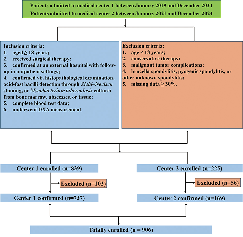Figure 1 Workflow of inclusion and exclusion process.

The diagnoses of tuberculosis spondylitis (TS) relied upon meticulous clinical evaluations, laboratory findings, and radiographic evidence. The inclusion criteria were: (1) aged ≥ 18 years; (2) received surgical therapy; (3) confirmed through surgery at an external hospital, but follow-up consultations were conducted in the outpatient setting. (4) confirmed through histopathological examination, detection of acid-fast bacilli using Ziehl–Neelsen staining, and/or the cultivation of Mycobacterium tuberculosis from culture specimens obtained from bone marrow, abscesses, or tissue.;²¹ (5) complete information of blood test data; (6) patients underwent DXA measurement.

BMD measurements of the hip and lumbar spine (L1-L4) were taken using DXA (Hologic Discovery, Hologic, Bedford, Massachusetts). The T-score was utilized as a reference to compare an individual’s BMD to the average BMD of healthy young adults with the same sex and ethnicity.²² The diagnoses of osteoporosis in patients were made based on the diagnostic criteria set by the World Health Organization (WHO).

The exclusion criteria were as follows: (1) age less than 18 years; (2) received conservative therapy; (2) complications with malignant tumors; (3) brucella spondylitis, pyogenic spondylitis or other unknown spondylitis; (4) missing data ≥ 30%.

Candidate Features

In this study, candidate features can be divided into two groups. One group includes general data such as age, gender, and body mass index (BMI). The other group comprises laboratory test parameters including, erythrocyte sedimentation rate (ESR), C-reactive protein (CRP), white blood cell count (WBC), neutrophil percentage (NEU%), lymphocyte percentage (LYM%), monocyte percentage (MONO%), eosinophil percentage (EOS%), basophil percentage (BASO%), neutrophil count (NEU), lymphocyte count (LYM), monocyte count (MONO), eosinophil count (EOS), basophil count (BASO), red blood cell count (RBC), hemoglobin (Hb), hematocrit (HCT), mean corpuscular volume (MCV), mean corpuscular hemoglobin (MCH), mean corpuscular hemoglobin concentration (MCHC), red cell distribution width (RDW), platelet count, mean platelet volume (MPV), platelet hematocrit (PHCT), platelet distribution width (PDW), immature granulocyte percentage (NRBC%), immature granulocyte count (NRBC), potassium (K), sodium (Na), chloride (Cl), bicarbonate (HCO3-), calcium (Ca), magnesium (Mg), inorganic phosphate (P), urea, creatinine, uric acid, estimated glomerular filtration rate (eGFR), triglycerides (TG), total cholesterol, high-density lipoprotein cholesterol (HDL-C), low-density lipoprotein cholesterol (LDL-C), apolipoprotein AI (apoAI), apolipoprotein B (apoB), lipoprotein(a) [Lp(a)], lactate dehydrogenase (LDH), creatine kinase (CK), free fatty acids (FFA), angiotensin-converting enzyme (ACE), retinol-binding protein (RBP), serum cystatin C, total bilirubin, direct bilirubin, indirect bilirubin, total protein, albumin, globulin, albumin/globulin ratio, aspartate aminotransferase (AST), alanine aminotransferase (ALT), AST/ALT ratio, gamma-glutamyl transferase (GGT), alkaline phosphatase (ALP), cholinesterase, and ammonia. Data from Center 1 were divided into a training set and an internal testing set in a 7.5:2.5 ratio, while data from Center 2 served as the external testing set.

Imbalanced Outcome Classes

Imbalanced target classes, a form of unbalanced data, can introduce bias in machine learning classifiers. A significant variation in target class distribution is frequently observed in metabolic datasets. To mitigate these challenges, we adopted the synthetic minority oversampling technique (SMOTE).²³ SMOTE enhances the fairness of data dispersion by generating synthetic data samples. This process involves identifying the K nearest neighbors, computing their distances, and augmenting these distances with random integers between 0 and 1.

Feature Selection and Data Preprocessing

Feature selection is a crucial step in machine learning and data analysis, as it identifies the most relevant predictors of a target variable. In our study, we applied three widely used feature selection techniques: LASSO (Least Absolute Shrinkage and Selection Operator), the Boruta algorithm, and Recursive Feature Elimination (RFE). Combining these methods offers more robust and accurate results. LASSO effectively identifies influential features, Boruta captures comprehensive predictive information without omitting relevant variables, and RFE iteratively removes less significant features. To verify the correlation between the selected variables, we used a heatmap. This combined approach improves the reliability and accuracy of identifying the most informative features related to osteoporosis in TS patients.

LASSO was a regularization technique that shrinks some coefficients to zero, thereby performing feature selection and reducing overfitting simultaneously.²⁴ The objective of LASSO was to minimize the sum of the residual error between the predicted and actual values of the target variable, subject to a constraint on the sum of the absolute values of the coefficients. The resulting model would have only a subset of coefficients that are deemed significant.

Boruta was an all-relevant feature selection algorithm that considers all possible features to identify those that contain valuable information related to the target variable.²⁵ Boruta works by comparing the importance of each feature to a set of randomized shadow features. Features that showed significantly higher importance than their corresponding shadows are deemed relevant and selected for further analysis. In contrast to other feature selection methods that aim to identify a minimal optimal subset of features, Boruta identified all relevant features associated with osteoporosis in TS patients.

RFE was a simple yet powerful technique that recursively eliminates less important features from the dataset to identify the most informative ones.²⁶ RFE assigned scores to each feature and eliminates those with the lowest scores. It then creates a new model with the remaining features and repeats the process until it reaches the desired number or until a stopping criterion is met. By iteratively eliminating the weakest features, RFE identified the most important predictors of the target variable that are associated with osteoporosis in TS patients.

The data was preprocessed by standardizing the features using a StandardScaler, ensuring that each feature had a mean of 0 and a standard deviation of 1. Missing values in the dataset were imputed using the Multiple Imputation by Chained Equations (MICE) method, which iteratively models each feature with missing values as a function of the other features, providing robust and reliable imputations.²⁷

Model Development

The supervised machine learning (ML) algorithms leverage training data to create a function (f) that maps input variables/features (X) to output/target (Y). The use of “labeled” training data sets is a common characteristic of supervised ML platforms, providing either qualitative or quantitative output. The labeled nature of these data sets during the training phase is crucial as it enables the ML model to mimic the input data, allowing the model to distinguish new inputs based on previously learned training parameters.

To develop and compare prediction models, various algorithms were employed. The construction of prediction models involved the implementation of the following methods: logistic regression (LR), extreme gradient boosting (XGBoost), light gradient boosting machine (LightGBM), random forest (RF), decision tree (DT), support vector machine classifier (SVC), k-nearest neighbors (KNN), and Gaussian naive Bayes (GNB). All prediction models were developed using Python 3.9. In addition, we also developed ensemble models using different combinations of the classifiers mentioned above using a soft voting strategy.

Hyperparameters are critical components of learning algorithms that must be predefined before model training and fitting. To optimize algorithm performance, the process of hyperparameter tuning involves selecting the optimal set of hyperparameters. In this study, we employed a nested cross-validation (CV) scheme and grid search algorithm to fine-tune the hyperparameters of all models during the training phase.²⁸ The process employs a nested cross-validation framework comprising two layers: an inner 5-fold loop for hyperparameter optimization via grid search and an outer 4-fold loop to assess the generalized performance of the tuned model on held-out data. The hyperparameter search space, including parameter ranges and sampling strategies, is detailed in Supplementary Table 1.

After configuring the parameters for each classifier, we assessed the performance of the model using different metrics. We visually represented the discrimination and agreement between actual and predicted values by plotting the Receiver Operating Characteristic (ROC) curve and Calibration plot, respectively. Additionally, we conducted Decision Curve Analysis to evaluate the clinical usefulness of the model. The ROC curve measures a classifier’s ability to distinguish between positive and negative classes, and the area under the curve (AUC) provides an indicator of its performance. The calibration plot assesses the agreement between predicted and observed probabilities across various predicted probability ranges. Through Decision Curve Analysis (DCA), we compared the model’s decision-making performance with alternative strategies to determine its clinical net benefit.

Model Selection and Threshold Tuning

To optimize model performance, threshold tuning was performed using the TunedThresholdClassifierCV tool from the sklearn library.²⁹ LR was chosen as the base model for its interpretability and efficiency. This tuning process was integrated into a repeated stratified k-fold cross-validation framework with 5 splits and 50 repeats to ensure robustness and address class imbalance. The primary aim was to maximize the F1-score, a balanced measure of precision and recall, while also evaluating clinically relevant metrics such as sensitivity, specificity, positive predictive value (PPV), and negative predictive value (NPV). These metrics were calculated confusion matrix. In addition, supplementary metrics like accuracy, balanced accuracy, Brier score, and log loss were included to offer a comprehensive view of the model’s performance. This approach ensured that the final model was both statistically robust and clinically relevant, particularly in decision-making scenarios where threshold values significantly impact outcomes. (Figure 2)

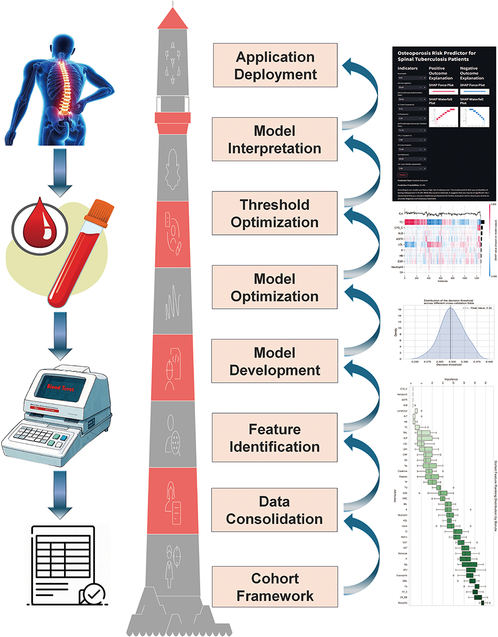Figure 2 Workflow of whole study.

Model Interpretation

In clinical applications, it is crucial to develop machine learning (ML) models that are interpretable and transparent, providing valuable insights for clinical practice. One significant challenge in achieving this goal is the “black-box problem”, where models are difficult to interpret, making it unclear why a specific prediction is made for a particular patient cohort. To enhance interpretability, we employed two methods: SHapley Additive exPlanations (SHAP).³⁰ By utilizing SHAP, we computed feature importance scores, which indicate the average marginal contribution of each feature to every prediction. The term “marginal” refers to the difference between the actual predicted value and a base value used as a reference. This calculation draws inspiration from coalitional game theory, allowing us to gain a deeper understanding of the model’s inner workings and the impact of individual features on its predictions.

Web Application Deployment

To ensure the easy and effective utilization of our chosen optimal model, we created a user-friendly web application utilizing the Python Flask web application development framework and popular frontend techniques.³¹ This web-based interface enables clinical practitioners and researchers to access and interact with the model in a simple and seamless manner. Our intention is to promote the adoption and usage of the model in real-world clinical settings by offering a freely accessible and user-friendly interface. Furthermore, we have implemented appropriate security measures within the web application to safeguard confidential patient data and maintain data privacy. These measures prioritize protecting sensitive information and ensuring that only authorized individuals have access to the data.

Statistical Analysis

Firstly, we assessed the normality of the data using the Shapiro–Wilks test. Continuous variables that followed a normal distribution were reported as mean values with standard deviation (SD), while continuous variables that did not follow a normal distribution were reported as median values with interquartile range. For the statistical analyses, we utilized R Version 4.2.1 (http://www.r-project.org). The ML models themselves were developed and analyzed using Python 3.9.5 and relied on the Scikit-learn packages (https://scikit-learn.org). To evaluate the performance of the models, we employed several evaluation metrics, including sensitivity, specificity, F1-score, and the area under the receiver operating characteristic curve (AUC). The AUC, in particular, measures how well the classifier can distinguish between positive and negative classes, providing a robust indicator of overall model performance.

Results

Study Participants

Out of a total of 906 patients, 60 (12 males, average age 67.2; 48 females, average age 67.2) were diagnosed with osteoporosis based on DXA measurements, while 846 were classified as non-osteoporotic (Supplementary Table 2). Patients with osteoporosis exhibited lower age-adjusted scores, bone mineral density, and physical activity levels compared to those without the condition. Additionally, the osteoporotic group had a higher prevalence of comorbidities. Although the average age was significantly higher in the osteoporotic group compared to the non-osteoporotic group, no significant differences were noted between the two groups regarding other factors.

Regarding demographic characteristics, the overall average age of participants was 47.6 years (SD = 20.1). The non-osteoporotic group, consisting of 846 participants, had an average age of 46.2 years (SD = 19.9). In contrast, the osteoporosis group, with 60 participants, had a significantly older average age of 67.2 years (SD = 9.1). The gender distribution showed that among all participants, 467 were female (51.5%) and 439 were male (48.5%). In the non-osteoporotic group, 419 were female (49.5%) and 427 were male (50.5%). However, the osteoporosis group had a higher proportion of females, with 48 females (80.0%) compared to 12 males (20.0%). This indicates a significant age difference and a notable gender imbalance in the osteoporosis group. Detailed demographic characteristics for participants, stratified by study center (Center 1 and Center 2), are documented in Supplementary Tables 3 and 4.

Variable Selection

We have implemented several feature selection tools to identify the most relevant predictors for osteoporosis. The LASSO regression analysis, illustrated in Figure 3A, showed how coefficients shrank with increasing regularization parameter log alpha. This method effectively removed less significant features, concentrating on the most important predictors. The cross-validation curve for LASSO, depicted in Figure 3B, plotted the mean squared error (MSE) against various λ values. Additionally, Figure 3C presents a bar plot of the non-zero feature coefficients retained by LASSO, ranked by absolute magnitude, clearly highlighting the most influential predictors: HB, eGFR, Platelets, ALT, and Creatinine.

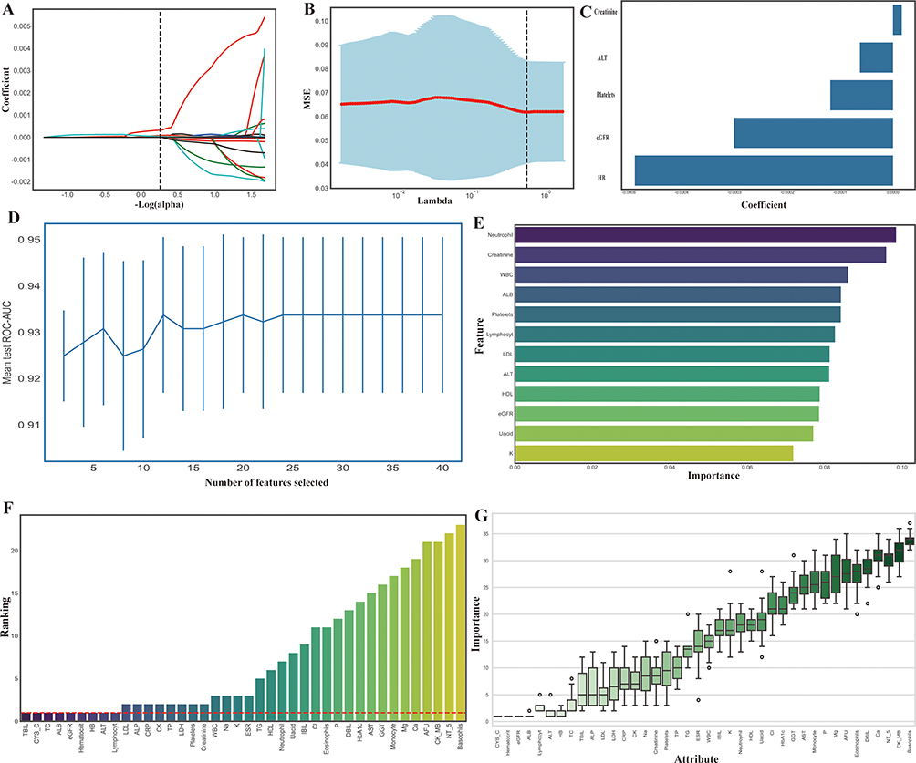Figure 3 Feature Selection. Feature Selection illustrates the process of identifying the most relevant features for the predictive model through several methodologies. (A): LASSO coefficient profiles demonstrate how the coefficients of each feature shrink as the regularization parameter log(α) increases, progressively eliminating less important features. (B): The cross-validation curve for LASSO, where the mean squared error (MSE) is plotted against different values of the regularization parameter λ, identifies the optimal λ at the minimum MSE to determine the selected features. (C): A bar plot of the non-zero feature coefficients retained by LASSO, ranked by their absolute magnitude, highlights the most influential predictors in the model. (D): The relationship between the number of features selected and model performance, measured by cross-validated Area Under the Curve (AUC), is depicted using Recursive Feature Elimination (RFE) based on a Support Vector Classifier (SVC). This plot reveals the trade-off between model complexity and predictive accuracy, with the optimal number of features identified at the peak AUC. (E): A horizontal bar chart ranks the features selected by the SVC-based RFE process, ordered by their importance scores or rankings, which reflect their contribution to the model’s classification performance. (F): The feature importance scores obtained through the Boruta feature selection algorithm are illustrated, which evaluate the relevance of each feature by comparing it to randomized shadow features, identifying the truly significant predictors. (G): A boxplot of the importance scores for the features selected by Boruta across multiple iterations (n=20) highlights the stability and variability of feature rankings and confirms the robustness of the selected features.

To complement the LASSO analysis, we implemented SVC-RFE, as shown in Figure 3D. This figure illustrates the relationship between the number of features selected and model performance, measured by cross-validated Area Under the Curve (AUC). The optimal number of features (n=12), identified at the peak AUC, balanced model complexity with predictive ability. Figure 3E presents a horizontal bar chart ranking the features selected by SVC-based RFE according to their importance scores, which reflect each feature’s contribution to classification performance. Notably, Neutrophils, Creatinine, WBC, ALB, and Platelets emerged as the most valuable predictors for osteoporosis. Lastly, we applied the Boruta feature selection algorithm, illustrated in Figure 3F, which evaluated feature relevance by comparing them to randomized shadow features. This method ensured that only the most significant features were included in the model. The Boruta algorithm identified several key predictors, including basophils, lymphocytes, hematocrit, hemoglobin (HB), total cholesterol (TC), estimated glomerular filtration rate (eGFR), cystatin C (CYS_C), albumin (ALB), alanine aminotransferase (ALT), and total bilirubin (TBIL). The robustness of the selected features was further confirmed through a boxplot of importance scores across multiple iterations (n=20), presented in Figure 3G. This visualization highlighted the stability and variability of feature rankings, with cystatin C, hematocrit and eGFR consistently ranking high in importance.

The univariate analysis conducted on the forty features revealed distinct differences in various health biomarkers (P < 0.05), as shown in Supplementary Figure 1. Neutrophil levels were elevated in the osteoporosis group, while hemoglobin (HB) levels were lower. The erythrocyte sedimentation rate (ESR) was significantly higher in individuals with osteoporosis compared to healthy controls. Lipid profiles demonstrated significant alterations in total cholesterol (TC) and low-density lipoprotein (LDL) levels in the osteoporosis group. Potassium (K) levels were also reduced in this group. Kidney function markers, including estimated glomerular filtration rate (eGFR) and cystatin C (CYS_C) levels, were significantly different, suggesting impaired kidney function in individuals with osteoporosis. Additionally, total protein (TP) and albumin (ALB) levels were lower in the osteoporosis group. Detailed comparison of biomarkers can be seen in Supplementary Table 5.

Above the selected features obtained from different methods, we selected Neutrophil (NEU), Hemoglobin (HB), Erythrocyte Sedimentation Rate (ESR), Total Cholesterol (TC), Low-Density Lipoprotein (LDL), Potassium (K), Estimated Glomerular Filtration Rate (eGFR), Cystatin C (CYS_C), Total Protein (TP), Albumin (ALB). Then we conducted correlation analysis in Figure 4, discovered significant strong correlation between selected features.

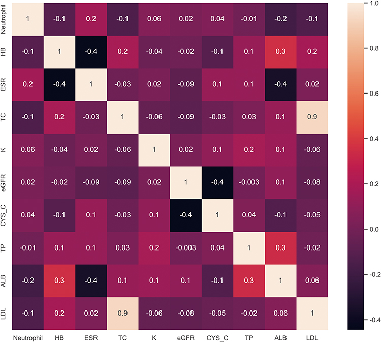Figure 4 Correlation analysis using Heatmap. This figure presents a heatmap of the correlation analysis conducted on the selected features. Each cell represents Pearson’s correlation coefficient between two features, with color intensity reflecting the strength of the correlation. Red cells denote positive correlations, while blue cells indicate negative correlations. The diagonal elements show the correlation of each feature with itself, always equal to 1. This heatmap provides a clear overview of feature relationships, enabling the identification of highly correlated features and their potential impact on model performance.

Feature Importance

We conducted a comprehensive analysis of feature importance across four tree-based models: Random Forest (RF), XGBoost (XGB), LightGBM (LGB), and Decision Tree (DT). In Figure 5A, the feature importances for the RF model are displayed, with eGFR, HB, and CYS_C emerging as the top three features, underscoring their significant impact on model predictions. The length of each bar indicates the relative importance of the corresponding feature, with longer bars signifying higher importance. Figure 5B illustrates the feature importances for the XGB model, where eGFR again ranks as the most important feature, followed by HB and CYS_C, like the RF model. This consistency across models suggests that these features play a crucial role in the prediction process. In Figure 5C, the feature importances for the LGB model are shown, where HB, ESR, and CYS_C take the top ranks, with a slight variation in feature ranking compared to RF and XGB. Figure 5D presents the feature importances for the DT model, where eGFR, HB, and CYS_C again emerge as the most influential features, reaffirming their critical role across all models analyzed. The consistency of eGFR, HB, and CYS_C as key predictors across all four models highlights their pivotal importance in the predictive tasks at hand.

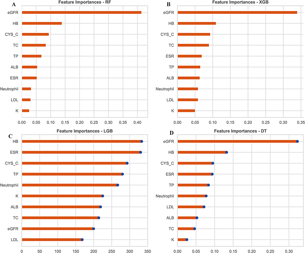Figure 5 Feature Importances Across Tree-based Models. (A): Bar chart showing the feature importances for the Random Forest model. (B): Bar chart showing the feature importances for the XGBoost model. (C): Bar chart showing the feature importances for the LightGBM model.(D): Bar chart showing the feature importances for the Decision Tree model.

Furthermore, we also utilized the LIME method to disclosure the importance of each feature. Figure 6A and B present bar charts that depict the feature importances as determined by the LIME method for two distinct machine learning models: Random Forest and XGBoost, respectively. Figure 6A shows that for the Random Forest model, the feature HB has the highest importance value, significantly exceeding other features such as ESR, TC, and eGFR. This suggests that HB plays a crucial role in the model’s predictions. The feature importances decrease progressively from HB to TP, indicating a varying degree of influence on the model’s outcomes. Figure 6B, representing the XGBoost model, mirrors a similar trend where HB is the most important feature, followed by TP and TC. However, the values for ESR and eGFR are relatively higher in the XGBoost model compared to the Random Forest model.

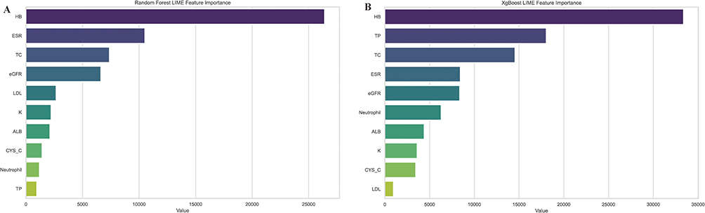Figure 6 Feature Importances in Machine Learning Models. (A) Bar chart representing the LIME feature importances for the Random Forest model. (B): Bar chart representing the LIME feature importances for the XGBoost model.

Resampling Techniques Validation

To assess the impact of various resampling techniques on model performance, we applied a range of strategies, including both over-sampling and under-sampling, to address class imbalance. We then compared the results of different resampling methods in combination with various algorithms to evaluate their effectiveness. Figure 7A, a scatter plot, presents the F1 scores for a variety of models including logistic regression, random forest, and support vector machines, each combined with sampling methods such as SMOTE, ROS, and ADASYN. The plot reveals that certain combinations of models and sampling techniques result in higher F1 scores, indicating superior performance. For instance, the combination of SVM with SMOTE-ENN shows a notably high F1 score, suggesting its effectiveness in handling imbalanced datasets. Figure 7B, a box plot, compares the F1 scores across different samplers including RUS, SMOTE-ENN, SMOTE, SMOTE-TOMEK, and ADASYN. This plot highlights the variability and central tendency of the F1 scores for each sampler, indicating that SMOTE-ENN and SMOTE-TOMEK generally yield higher scores, suggesting their reliability in improving model performance. Figure 7C, a bar chart, compares the mean F1 scores for various samplers, emphasizing the effectiveness of each method in handling imbalanced datasets. The chart clearly shows that SMOTE-ENN and SMOTE-TOMEK achieve higher mean F1 scores, indicating their superior performance in improving model accuracy compared to other methods like ADASYN and K-Means-SMOTE. Based on the above results, we chose smote for further analysis.

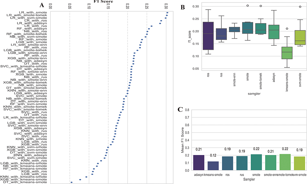Figure 7 Performance of Different Sampling Techniques (A): Scatter plot showing the F1 scores for various machine learning models combined with different sampling techniques. (B): Box plot comparing the F1 scores across different samplers. (C): Bar chart comparing the mean F1 scores for various samplers.

Performance of Classifiers

To screen the algorithm that has the best discrimination ability towards osteoporosis, we have carried out a series of analysis. Figure 8A presents a Receiver Operating Characteristic (ROC) curve, which is a graphical representation of the model’s ability to distinguish between classes. The curve shows the trade-off between sensitivity (true positive rate) and specificity (1 - false positive rate) across different threshold settings. The area under the curve (AUC) values are provided for each model, with LR showing the highest AUC of 0.826, indicating its superior performance in distinguishing between classes compared to other models such as XGB and (RF. Figure 8B depicts a calibration plot, which assesses how well the predicted probabilities align with the actual outcomes. The plot shows the fraction of positives (positive class: 1) against the mean predicted probability. The closer the plot follows the dotted line representing perfect calibration, the better the model’s predictions align with actual outcomes. Figure 8C illustrates decision analysis curve plot, which evaluates the clinical utility of the models at different threshold probabilities. The plot compares the net benefit of treating all patients versus treating none, with Logistic Regression showing a higher net benefit across most threshold probabilities, suggesting its potential effectiveness in clinical decision-making. Detailed assessments of these models, including their predictive accuracy, generalizability, are presented in Table 1.

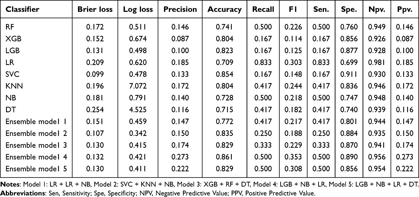Table 1 Detailed Information of Performance

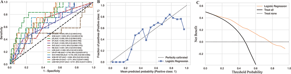Figure 8 Performance Metrics of Machine Learning Models. (A) This graph shows the ROC curves for various machine learning models, including Logistic Regression, XGBoost, and Random Forest. The plot includes AUC values for each model, providing a measure of their ability to distinguish between classes. (B): This plot is a calibration curve that compares the predicted probabilities of a model to the actual outcomes. The dotted line represents perfect calibration, and the plot shows how closely the Logistic Regression model’s predictions align with actual results. (C): The decision analysis curve plot evaluates the clinical utility of the models at different threshold probabilities. It compares the net benefit of treating all patients versus treating none, with Logistic Regression showing a higher net benefit across most threshold probabilities.

To assess the generalized predictive capability of the logistic regression (LR) algorithm, we tested it on an external dataset. As shown in Figure 9A, the ROC curve highlights the model’s ability to differentiate between classes effectively. The area under the curve (AUC) of 0.796 indicates robust discriminatory performance, significantly surpassing random chance. In Figure 9B, a net benefit analysis further evaluates the clinical utility of the model across varying threshold probabilities. The results reveal a consistently positive net benefit over a wide range of thresholds, underscoring its practical relevance. The narrow-shaded area, representing the uncertainty of the net benefit estimate, reinforces the model’s reliability and strengthens confidence in its performance. These findings collectively demonstrate the LR model’s potential for clinical application and its ability to generalize across datasets.

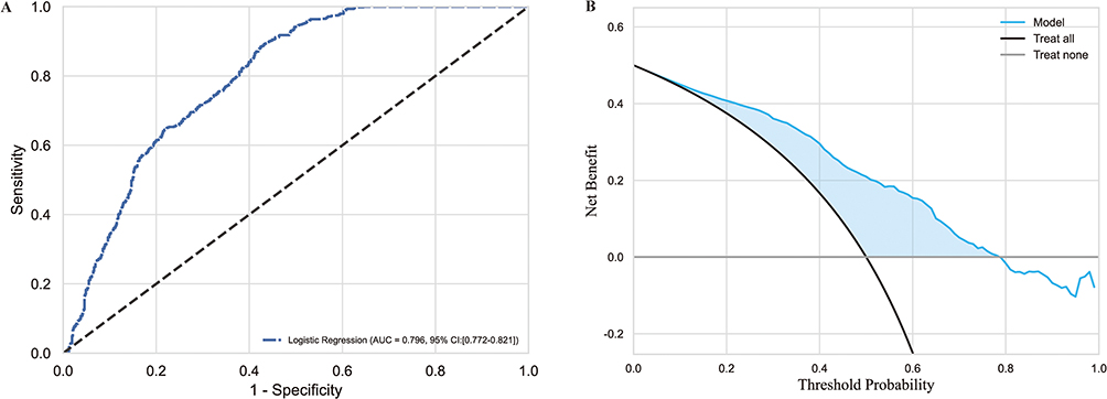Figure 9 Performance Evaluation of Logistic Regression Models. (A) This graph depicts the ROC curve for a logistic regression model, showing the trade-off between sensitivity and specificity. The curve illustrates the model’s ability to correctly identify positive cases compared to negative ones. (B): This plot presents a net benefit analysis for the logistic regression model, evaluating its clinical utility across different threshold probabilities. The plot includes a shaded area representing the confidence interval around the net benefit estimate.

Threshold Optimalization

The best-performing LR model initially yielded relatively low F1 scores. To address this, we implemented threshold tuning to enhance performance. Figure 10A illustrates box plots comparing key performance metrics—accuracy, balanced accuracy, F1 score, precision, recall, sensitivity, specificity, NPV, and PPV—across both training and testing datasets. While training scores marginally outperformed test scores, indicating slight overfitting, the balanced accuracy and F1 score demonstrated minimal variation between datasets. This consistency suggests the model effectively balanced the identification of both classes. Figure 10B presents box plots for the Brier score and negative log loss, which assesses the accuracy of probabilistic predictions. The distributions of these metrics were closely aligned across training and testing datasets, underscoring the model’s reliability in producing accurate and consistent predictions. Finally, Figure 10C depicts a density plot of the best decision threshold during tuning, revealing a peak at 0.32. This optimal threshold highlights a clear decision boundary, ensuring robust classification of new instances. Then we used 0.32 as the threshold and made cv-roc (cv=10) on the whole dataset as shown in Figure 11, revealed AUC=0.79.

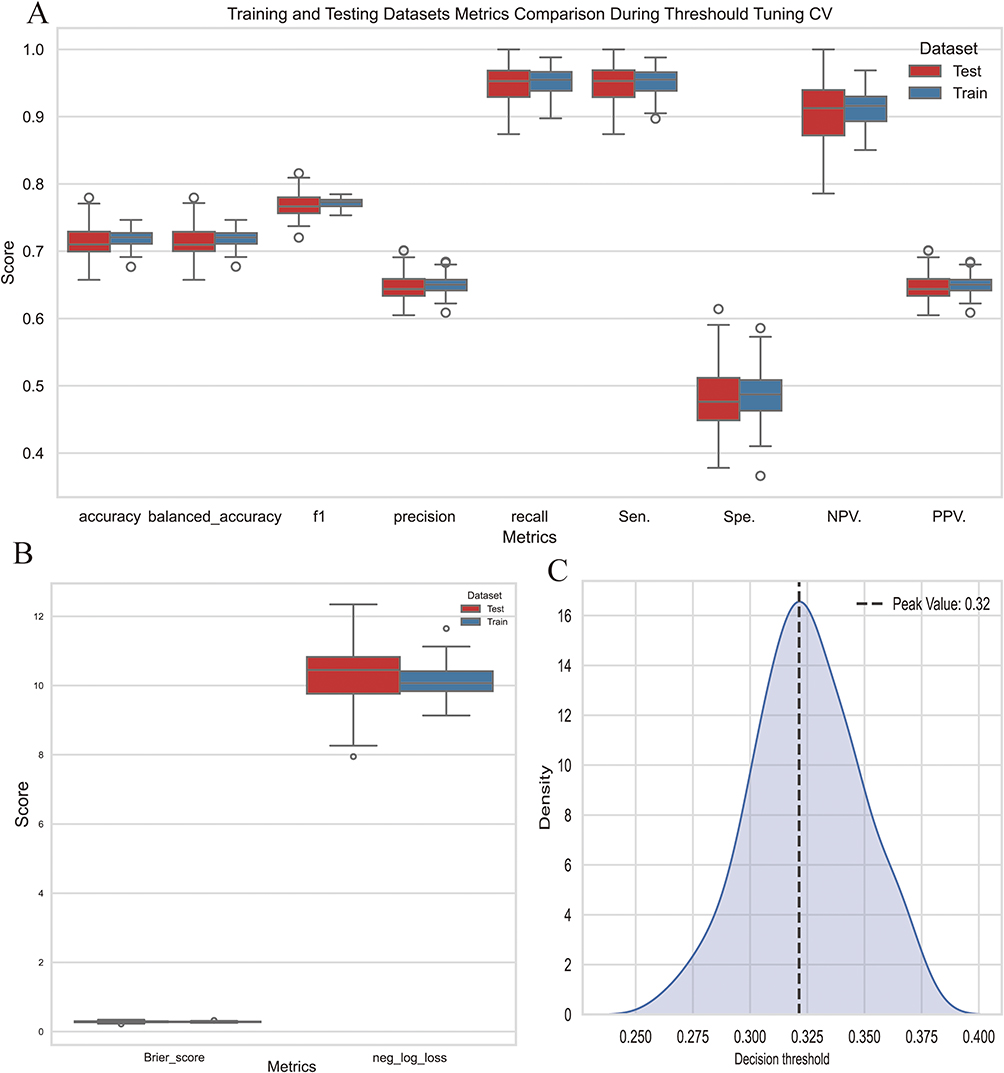Figure 10 Model Performance Metrics During Threshold Tuning Cross-Validation (A) Box plots comparing key performance metrics between training and testing datasets, including accuracy, balanced accuracy, F1 score, precision, recall, sensitivity, specificity, NPV, and PPV. (B): Box plots showing the Brier score and negative log loss for both training and testing datasets. (C): Density plot of the decision threshold, with a peak indicating the optimal threshold value.

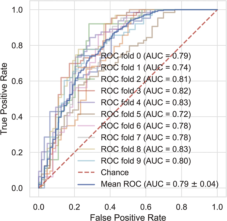Figure 11 10-fold cross-validation receiver operator characteristics curve (ROC). The ROC curve was derived from a 10-fold cross-validation process, a method designed to evaluate model performance across multiple subsets of data. This approach ensures a more comprehensive assessment of the model’s predictive capabilities by averaging its performance over different data partitions. The ROC curve illustrates the relationship between the true positive rate (sensitivity) and the false positive rate (1 - specificity) across various classification thresholds. This visualization highlights the trade-off between sensitivity and specificity, offering a clear depiction of the model’s ability to distinguish between positive and negative instances. By employing 10-fold cross-validation, the evaluation becomes more robust, minimizing the impact of data variability or potential bias inherent in a single train-test split. The resulting ROC curve not only provides a reliable measure of the model’s generalization ability but also assists in identifying an optimal classification threshold for practical application.

Model Interpretation

To enhance the clinical applicability of the model, we applied the SHAP method to identify key features influencing osteoporosis screening predictions in patients with TS. SHAP values were used to assess the importance of features and the prediction accuracy of the algorithm. Interpreting these values involves examining both the magnitude and the sign of each feature’s SHAP value. The x-axis of the plots represents the magnitude, while colors (red for positive and blue for negative) indicate the sign. Features are ranked according to their contribution to the predictions, with larger values signifying stronger impacts. The analysis revealed how biomarker contributions interact with the model’s decision-making process. Figure 12A, a SHAP beeswarm plot, illustrates the impact of each feature on the model’s output. The plot shows that features such as eGFR and HB have the most significant positive impact, as indicated by their high SHAP values on the right side of the plot. In contrast, features like TP have a more neutral or slightly negative impact, as shown by their positions closer to or on the left side of the zero line. Figure 12B, a decision plot, visualizes the distribution of SHAP values across all features for different model output values. The plot reveals that features like eGFR and HB have a wider distribution of SHAP values, suggesting a more variable impact across different model predictions. In Figure 12C, which represents an osteoporosis case, ALB (+0.24) and TP (+0.01) were identified as key risk factors, positively influencing the prediction of osteoporosis. Additionally, eGFR (+0.55), HB (+0.38), and K (+0.27) demonstrated the most substantial positive contributions to the predictions, while LDL (−0.06) exhibited a minor negative impact, suggesting a protective effect. The color gradient and distribution of data points highlighted the variability in biomarker effects across individual samples. In contrast, the normal case (Figure 12D) revealed that declining eGFR (106.64, −0.44) and HB (145, −0.39) were associated with reduced prediction confidence, as indicated by their downward trajectories on the scale (−1.50 to 0.25). Elevated levels of CYS_C (SHAP value: −0.16) and ESR (−0.41) were identified as significant negative drivers, further reducing the likelihood of osteoporosis. These findings underscore the differential roles of biomarkers in disease prediction and emphasize the importance of context-specific interpretations in clinical decision-making.

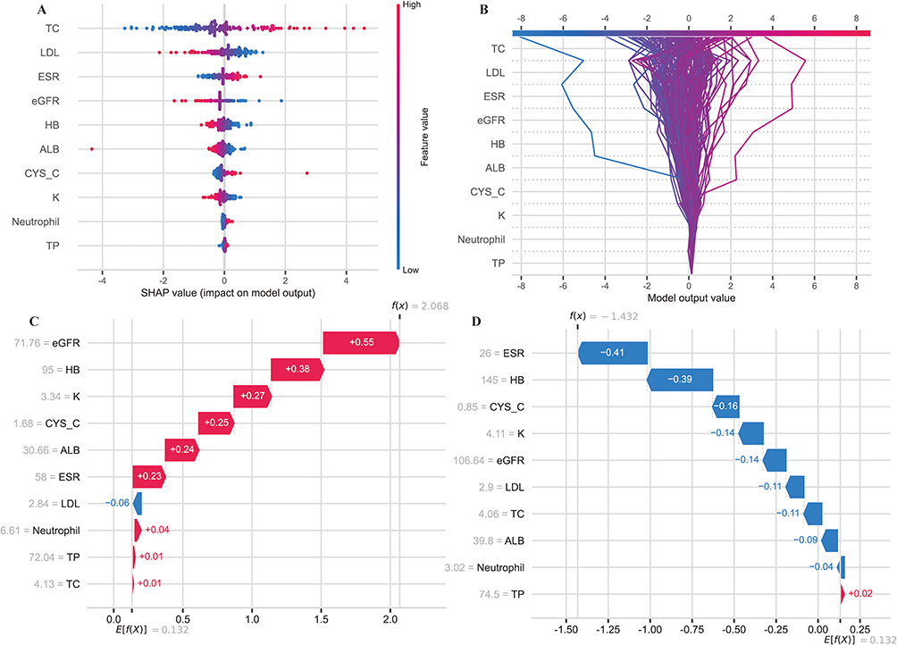Figure 12 Model general interpretation. General interpretation of the model’s performance and behavior obtained from training. (A): Feature importance ranking as indicated by SHAP. The bar plot describes the importance of each covariate in the development of the final prediction model. (B): The figure displays the key features contributing to the model’s predictions for each functional cluster. It includes raw data labels for each feature, a SHAP value plot showing the distribution of SHAP values across all cases, and an x-axis representing the impact of a feature on the predicted functional status classification. The color of a data point represents its feature value, while the vertical heat map highlights high feature values in red. (C): The waterfall plot illustrates the progression of feature contributions (SHAP values) for a representative high-risk osteoporosis case (D): The waterfall plot delineates the additive contributions of features to a representative normal case.

Model Online Development

To enhance clinical practicality and facilitate bedside usage, we have developed a user-friendly online application that incorporates the trained model. This application not only provides predictions but also offers interpretations of the results generated by the model. It is freely accessible and can be conveniently utilized by healthcare professionals (https://ts-osteoporosis.streamlit.app/) (Figure 13).

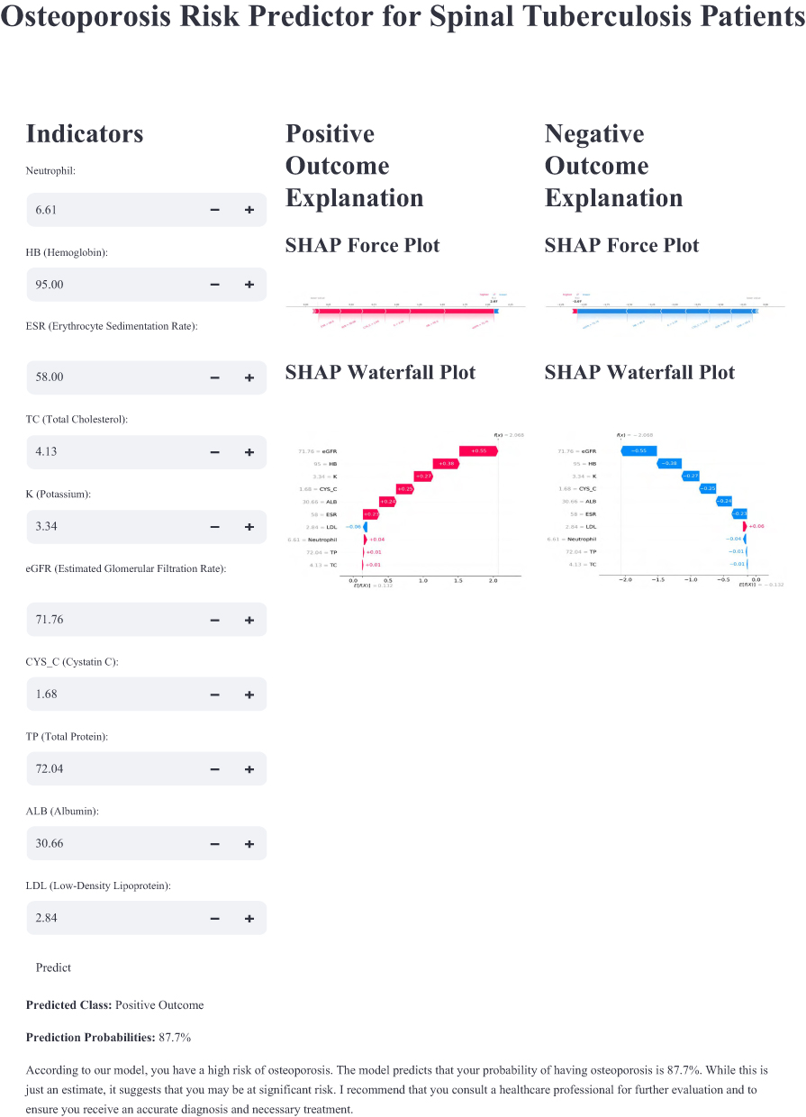Figure 13 Online free web application. The screenshot of web application which runs the developed model in backend.

Discussion

Tuberculosis spondylitis (TS), a rare condition characterized by an insidious onset and slow progression, is more prevalent in regions with high rates of pulmonary tuberculosis. The thoracic and thoracolumbar spine are the most affected sites. TS can lead to severe complications, including invasion of adjacent vertebral structures and intervertebral discs, resulting in Pott’s disease. This condition often manifests as abscess formation, spinal cord compression, vertebral collapse, and significant kyphotic deformity.³² In our previously published study, we developed a machine learning model to predict prolonged length of stay (PLOS) in hospitals following surgery for TS patients, employing feature selection techniques such as LASSO, RFE, correlation analysis, and permutation importance.³³ Building upon this foundation, the current study aims to advance clinical decision-making by developing an interpretable machine learning model specifically for screening osteoporosis in TS patients. In this study, osteoporosis was diagnosed in 60 out of 906 patients based on DXA measurements, while the remaining 846 patients were classified as non-osteoporotic. The osteoporotic group, predominantly older females, exhibited lower bone mineral density, reduced physical activity, and a higher prevalence of comorbidities. While our previous work centered on predicting PLOS using inflammatory markers (eg, C-reactive protein) and imaging-derived features, this study shifts focus to osteoporosis prediction. Employing advanced feature selection techniques—including LASSO regression, SVC-RFE, and Boruta—we identified hemoglobin (HB), estimated glomerular filtration rate (eGFR), and cystatin C (CYS_C) as novel biomarkers strongly associated with osteoporosis risk. Tree-based machine learning models further corroborated the importance of these factors, consistently prioritizing HB, eGFR, and CYS_C as the most influential predictors in osteoporosis risk stratification. To mitigate class imbalance, resampling techniques such as SMOTE were employed, significantly enhancing model performance. Prior ML studies focused on postmenopausal or age-related osteoporosis using imaging or genetic data. In contrast, our model targets TS-specific pathways by incorporating inflammation (ESR), renal function (CYS_C), and nutritional markers (HB) reflective of TB-associated metabolic dysregulation. This approach avoids reliance on DXA, which is often inaccessible in TB-endemic regions, and provides a scalable solution for low-resource settings.

Machine learning models have demonstrated significant potential in osteoporosis risk screening, outperforming conventional machine learning models and clinical tools. For instance, a deep learning model developed for osteoporosis risk prediction achieved AUC values of 0.851 and 0.922 for different bone mineral density sites using the NHANES dataset, and 0.827 and 0.912 using the KNHANES dataset, highlighting its robust performance across diverse populations.³⁴ Similarly, AI applications leveraging CT imaging for osteoporosis classification reported AUCs ranging from 0.582 to 0.994, reflecting variability in effectiveness depending on the specific AI model and imaging technique employed.³⁵ Radiomics-based machine learning approaches have also shown promise, with a study utilizing abdomen-pelvic CT radiomics features achieving AUCs of 95.9% and 96.0% in training and validation cohorts, respectively, underscoring high predictive accuracy for femoral osteoporosis.³⁶ Furthermore, various AI models, including artificial neural networks (ANN), support vector machines (SVM), and random forests, have consistently outperformed traditional methods, with AUCs ranging from 0.762 to 0.901 across different datasets.³⁷ Notably, opportunistic screening using deep learning models applied to chest radiographs achieved AUCs of 0.91 and 0.88 in internal and external test sets, respectively, suggesting their potential for widespread osteoporosis screening in routine clinical settings.³⁸ These findings collectively emphasize the transformative role of AI in enhancing osteoporosis risk prediction and screening, offering a pathway for more accurate and accessible diagnostic tools. In this research, logistic regression achieved the highest area under the curve (AUC) of 0.826, with external validation confirming the model’s robustness (AUC=0.796).

Class imbalance presented a significant challenge in our study, as classifiers employing a default decision threshold of 0.5 frequently underperformed on imbalanced datasets, particularly when the minority class was the primary focus. To address this, threshold tuning—a critical process in machine learning—was employed to adjust the decision threshold used by classifiers, thereby improving their performance in imbalanced data scenarios. This adjustment was essential for enhancing the accuracy and reliability of machine learning models across various applications. By optimizing the threshold, we ensured that the models could better distinguish between classes, even when one class was underrepresented. This approach not only improved the predictive performance but also provided a more robust framework for handling imbalanced datasets, which is a common issue in medical research. The findings underscore the importance of threshold tuning as a practical strategy to mitigate the effects of class imbalance, ultimately contributing to more reliable and generalizable machine learning models in clinical and biomedical applications. To address this, adjusting the decision threshold emerged as a practical and effective solution, significantly improving classification performance by reducing the misclassification rate of the minority class without the need for model retraining or data resampling.³⁹ Through threshold tuning with cross-validation, we identified that most optimal thresholds clustered around 0.32, corresponding to the highest performance peak. This approach proved especially valuable in optimizing critical metrics such as precision, recall, and false alarm rates, which are crucial in applications like predictive monitoring. The successful implementation of threshold optimization strategies across diverse domains highlights their efficacy in balancing these metrics.⁴⁰ By addressing these challenges, our findings emphasize the potential to enhance the robustness and real-world applicability of machine learning models, offering a pathway to more reliable and accurate predictive outcomes in medical research.

A critical consideration in osteoporosis prediction is the undeniable influence of advancing age, a primary and well-established risk factor [cite landmark epi studies]. Our demographic data confirms a significant age difference between the OP and Normal cohorts in our study. However, during our model development process, which included initial feature selection incorporating age and sex, these demographic variables were not retained among the top predictors by the algorithm. Furthermore, subsequent exploratory analyses forcing the inclusion of age and sex alongside the selected biomarkers did not yield an improvement in model performance (AUC) on our current dataset, with preliminary cross-validation suggesting potentially slightly lower predictive accuracy compared to the biomarker-only model. This counterintuitive result likely does not reflect the true biological or clinical importance of age but may instead be an artifact stemming from the specific limitations of this dataset, including the relatively modest sample size, the pronounced class imbalance, and potential complex interactions between variables that our models struggled to capture effectively within this data regime. Consequently, while our study focused on identifying a potential biomarker signature, this finding underscores a significant limitation: the inability of our current analysis, constrained by data characteristics, to fully integrate the known dominant effect of age. It highlights the imperative for future research using larger, more robust datasets where the crucial contributions of age and sex can be reliably modeled alongside biomarkers to develop clinically comprehensive predictive tools.

We found neutrophil was the key element related osteoporosis in our research. Neutrophils play a critical role in fostering a proinflammatory environment that drives osteoporotic bone remodeling. In aging individuals, neutrophils exhibit diminished chemotaxis, phagocytosis, and apoptosis, which may worsen bone deterioration.⁴¹ Elevated neutrophil levels have been shown to inhibit the synthesis of mineralized extracellular matrix by bone marrow stromal cells, potentially impairing bone regeneration and contributing to the progression of osteoporosis.⁴² Furthermore, systemic inflammation in osteoporosis is reflected by increased neutrophil-to-lymphocyte ratio (NLR) and platelet-to-lymphocyte ratio (PLR), both of which are significantly elevated in affected individuals. Notably, these markers are particularly higher in postmenopausal women with osteoporosis, underscoring their potential utility as non-invasive screening tools for the disease.⁴³ Together, these findings highlight the intricate interplay between neutrophil dysfunction, systemic inflammation, and bone loss, offering insights into potential diagnostic and therapeutic avenues for osteoporosis.

Furthermore, bone quality and fracture risk are significantly influenced by anemia, particularly in older adults, who exhibit poorer bone quality and a higher susceptibility to fractures. Studies have demonstrated that anemic individuals often present with lower bone mineral density (BMD) and an elevated risk of fractures, a trend that is especially pronounced in aging populations.^44,45 These were in line with our findings. Furthermore, hemolytic anemia has been specifically associated with an increased risk of osteoporosis, likely due to heightened hematopoietic stress and the impact of dysregulated iron metabolism on bone health.⁴⁶ In patients with chronic kidney disease (CKD), anemia is highly prevalent and closely linked to disruptions in bone metabolic biomarkers. Emerging evidence suggests that therapeutic interventions targeting bone metabolic disorders may offer a dual benefit by concurrently managing anemia in this patient population.⁴⁷ These findings underscore the intricate interplay between anemia and bone health, highlighting the need for integrated approaches to mitigate fracture risk and improve outcomes in affected individuals.

Increased ESR in osteoporosis has been consistently observed in postmenopausal women, with studies demonstrating higher levels in those with osteoporosis compared to individuals with normal bone mineral density (BMD) or osteopenia, suggesting a connection between elevated ESR and systemic inflammation in this condition.^48,49 This inflammatory response is further supported by the elevation of additional markers, such as C-reactive protein (CRP), which are known to associate with osteoporosis; however, CRP was not identified as a key predictive feature in our analysis.⁵⁰ While both ESR and CRP are utilized to assess systemic inflammation, CRP is generally regarded as a more sensitive indicator. However, in our cohort, most TS-osteoporosis cases were observed in women, contrasting with prior research that has predominantly associated elevated inflammatory markers (eg, CRP) with impaired bone quality in older male populations. While this relationship is well-documented in men, its significance in female cohorts remains less clearly established.⁵⁰ These findings underscore the role of systemic inflammation in the pathophysiology of osteoporosis and highlight the potential utility of inflammatory markers in understanding bone health and disease progression.

Our findings revealed a notable relationship between lipid profiles and bone health, with dyslipidemia emerging as a significant factor influencing bone integrity. Elevated levels of TC and LDL were associated with reduced bone mass and increased fracture risk, likely mediated by heightened oxidative stress and systemic inflammation. These conditions promote osteoclastic activity while impairing bone formation, thereby disrupting bone homeostasis.⁵¹ Lipid metabolism plays a pivotal role in this process, as imbalances in lipid levels can modulate immune cell activity and the secretion of inflammatory factors, driving osteoclast differentiation and bone resorption, which contribute to osteoporosis.⁵² Notably, specific lipid profiles within the bone marrow, such as elevated triglycerides and altered fatty acid compositions, have been identified as potential biomarkers for osteoporosis, offering promising avenues for early diagnosis and intervention. The interplay between lipid-induced inflammation and oxidative stress further underscores their role as key mechanisms that inhibit osteogenesis and accelerate bone resorption, exacerbating osteoporosis progression. Additionally, dietary lipids significantly impact bone health, with certain unsaturated fats, such as omega-9, potentially enhancing bone strength and architecture, while diets high in saturated fats may worsen osteoporosis.⁵³ Collectively, these findings highlight the intricate connections between lipid metabolism, inflammation, oxidative stress, and bone health, providing valuable insights into the pathogenesis of osteoporosis and identifying potential therapeutic targets.

Our findings revealed that renal function-related indicators were associated with osteoporosis in TS patients, suggesting a potential link between chronic kidney disease and bone health. Chronic Kidney Disease-Mineral and Bone Disorder (CKD-MBD), a systemic condition characterized by dysregulation of calcium, phosphorus, parathyroid hormone (PTH), and vitamin D metabolism, likely contributes to bone abnormalities, increased fracture risk, and cardiovascular complications in this population.^54,55 These metabolic disturbances are directly tied to the progressive decline in kidney function. Renal osteodystrophy, a component of CKD-MBD, encompasses bone diseases such as osteitis fibrosa, osteomalacia, and adynamic bone disorder, all stemming from mineral metabolism imbalances caused by impaired kidney function.^54,56 The kidney plays a pivotal role in maintaining bone health by regulating calcium and phosphate homeostasis, which are critical for bone mineralization. Additionally, the kidney synthesizes essential substances like 1,25(OH)2D3 and erythropoietin, which are vital for bone formation and repair.⁵⁷ Kidney donation, while lifesaving, can induce acute disruptions in mineral metabolism, including reduced phosphate levels and alterations in bone-related hormones, potentially impacting bone health.⁵⁸ Post-transplantation, mineral and bone disorders may persist or evolve due to changes in kidney function and the effects of immunosuppressive therapy, necessitating continuous monitoring and management to mitigate complications.⁵⁹

It is crucial to interpret these findings within the specific clinical context of Tuberculous Spondylitis (TS). Unlike primary osteoporosis, where the focus is often on predicting long-term minimal trauma fractures in the general population, osteoporosis in TS is predominantly a secondary phenomenon driven by a distinct pathophysiology involving chronic inflammation, malnutrition, and immobilization associated with the infection itself. Consequently, the primary clinical implication shifts towards peri-operative risks, such as instrumentation failure and compromised fusion healing following spinal surgery. While we employed the standard WHO definition for osteoporosis diagnosis based on BMD T-scores, the underlying mechanisms and the immediate clinical relevance differ significantly from age-related bone loss. Our biomarker-based model attempts to capture aspects of this specific TS-related pathophysiology. Therefore, readers should consider that this tool is designed for risk stratification within this unique, high-risk patient group facing potential surgical intervention, rather than as a direct substitute for general population fracture risk calculators like FRAX^®, whose calibration may not fully extend to this specific secondary cause of osteoporosis.

We developed a user-friendly, freely accessible online calculator to integrate our predictive model into clinical practice. This tool enables healthcare professionals to easily input key demographic and laboratory data, generating real-time predictions of osteoporosis risk in patients with tuberculosis spondylitis. Designed for simplicity and efficiency, the calculator simplifies decision-making by offering immediate, actionable insights without requiring specialized software or extensive training. The interface also features intuitive visualizations and explanations based on our machine learning models, improving the transparency and reliability of predictions. By providing open access to this tool, we aim to help clinicians identify high-risk patients more quickly, optimize surgical planning, and enhance patient outcomes. This online calculator extends our research’s practical application, fostering the adoption of evidence-based practices and bridging the gap between complex analytical models and daily clinical use. Envisioning the clinical impact, this biomarker-based tool could transform decision-making in TS patients by enabling preoperative risk stratification, such as selecting augmented fixation techniques or initiating bone-protective therapies to mitigate fracture risks. For instance, a high-risk prediction might prompt conservative management delays or targeted interventions, potentially reducing complications like implant failure. However, as a screening aid with inherent limitations in sensitivity, it should complement BMD assessments and existing tools like FRAX, with future validations needed to refine its integration into routine practice.

Limitations

This study has several limitations that must be considered. First, its retrospective design may introduce selection bias, as it relies on existing records which may not capture all relevant variables. Second, the study was conducted at a single medical center in northwestern China, potentially limiting the generalizability of the findings to other populations and regions. Additionally, while we employed SMOTE to address class imbalance, the generation of synthetic samples may not fully replicate the complexity of real-world data, possibly affecting model performance. The reliance on routine blood test data, while practical, may omit other important predictors of osteoporosis that were not available in the dataset. Furthermore, although we utilized multiple feature selection methods to identify key predictors, there is a possibility of residual confounding factors influencing the results. Finally, the external validation was performed on a limited dataset, and larger-scale studies are necessary to confirm the robustness and applicability of the developed models across diverse clinical settings.

Conclusions

In conclusion, our study successfully developed and validated machine learning models that predict osteoporosis in patients with tuberculosis spondylitis using accessible demographic and blood test data. The logistic regression model demonstrated strong predictive performance, supported by external validation, and its interpretability was enhanced through explainable AI techniques. By reducing dependence on DXA measurements, these models offer a practical and efficient tool for early osteoporosis screening, which can inform surgical decisions and improve patient outcomes in clinical settings. The deployment of an online application further facilitates the integration of this predictive tool into routine healthcare practices. Future research should focus on expanding the dataset, incorporating additional predictive factors, and conducting multicenter studies to enhance the generalizability and accuracy of the models. Ultimately, leveraging machine learning in this context holds promise for advancing personalized medicine and optimizing the management of osteoporosis in TS patients.

References

1. Trecarichi EM, Di Meco E, Mazzotta V, Fantoni M. Tuberculous spondylodiscitis: epidemiology, clinical features, treatment, and outcome. Eur Rev Med Pharmacol Sci. 2012;16(2):58–72.
2. Su SH, Tsai WC, Lin CY, et al. Clinical features and outcomes of spinal tuberculosis in southern Taiwan. J Microbiol Immunol Infect. 2010;43(4):291–300. doi:10.1016/S1684-1182(10)60046-1
3. de la Rua-Domenech R. Human mycobacterium bovis infection in the United Kingdom: incidence, risks, control measures and review of the zoonotic aspects of bovine tuberculosis. Tuberculosis. 2006;86(2):77–109. doi:10.1016/j.tube.2005.05.002
4. Rao H, Shi X, Zhang X. Using the kulldorff’s scan statistical analysis to detect spatio-temporal clusters of tuberculosis in Qinghai Province, China, 2009-2016. BMC Infect Dis. 2017;17(1):578. doi:10.1186/s12879-017-2643-y
5. Sai Kiran NA, Vaishya S, Kale SS, Sharma BS, Mahapatra AK. Surgical results in patients with tuberculosis of the spine and severe lower-extremity motor deficits: a retrospective study of 48 patients. J Neurosurg Spine. 2007;6(4):320–326. doi:10.3171/spi.2007.6.4.6
6. Mak KC, Cheung KM. Surgical treatment of acute TB spondylitis: indications and outcomes. Eur Spine J. 2013;4(Suppl 4):603–611. doi:10.1007/s00586-012-2455-0
7. Yagi M, Fujita N, Tsuji O, et al. Low bone-mineral density is a significant risk for proximal junctional failure after surgical correction of adult spinal deformity. Spine. 2018;43(7):485–491. doi:10.1097/Brs.0000000000002355
8. Pinter ZW, Monsef JB, Salmons HI, et al. Does preoperative bone mineral density impact fusion success in anterior cervical spine surgery? A prospective cohort study. World Neurosurg. 2022;164:e830–e834. doi:10.1016/j.wneu.2022.05.058
9. Zaidi Q, Danisa OA, Cheng W. Measurement techniques and utility of Hounsfield unit values for assessment of bone quality prior to spinal instrumentation: a review of current literature. Spine. 2019;44(4):E239–E244. Spine (Phila Pa 1976). doi:10.1097/BRS.0000000000002813
10. Kwon BK, Elgafy H, Keynan O, et al. Progressive junctional kyphosis at the caudal end of lumbar instrumented fusion: etiology, predictors, and treatment. Spine. 2006;31(17):1943–1951. doi:10.1097/01.brs.0000229258.83071.db
11. Yu F, Xia W. The epidemiology of osteoporosis, associated fragility fractures, and management gap in China. Arch Osteoporos. 2019;14(1):32. doi:10.1007/s11657-018-0549-y
12. Zeng Q, Li N, Wang Q, et al. The prevalence of osteoporosis in China, a nationwide, multicenter DXA survey. J Bone Miner Res. 2019;34(10):1789–1797. doi:10.1002/jbmr.3757
13. Siris ES, Adler R, Bilezikian J, et al. The clinical diagnosis of osteoporosis: a position statement from the national bone health alliance working group. Osteoporos Int. 2014;25(5):1439–1443. doi:10.1007/s00198-014-2655-z
14. Pinheiro MB, Oliveira J, Bauman A, Fairhall N, Kwok W, Sherrington C. Evidence on physical activity and osteoporosis prevention for people aged 65+ years: a systematic review to inform the WHO guidelines on physical activity and sedentary behaviour. Int J Behav Nutr Phys Act. 2020;17(1):150. doi:10.1186/s12966-020-01040-4
15. Thomsen K, Jepsen DB, Matzen L, Hermann AP, Masud T, Ryg J. Is calcaneal quantitative ultrasound useful as a prescreen stratification tool for osteoporosis? Osteoporos Int. 2015;26(5):1459–1475. doi:10.1007/s00198-014-3012-y
16. Cheng X, Zhao K, Zha X, et al. Opportunistic screening using low-dose CT and the prevalence of osteoporosis in China: a nationwide, multicenter study. J Bone Miner Res. 2021;36(3):427–435. doi:10.1002/jbmr.4187
17. Wu HZ, Zhang XF, Han SM, et al. Correlation of bone mineral density with MRI T2* values in quantitative analysis of lumbar osteoporosis. Arch Osteoporos. 2020;15(1):18. doi:10.1007/s11657-020-0682-2
18. Inui A, Nishimoto H, Mifune Y, et al. Screening for osteoporosis from blood test data in elderly women using a machine learning approach. Bioengineering. 2023;10(3):277. doi:10.3390/bioengineering10030277
19. Zeitlin J, Parides MK, Lane JM, Russell LA, Kunze KN. A clinical prediction model for 10-year risk of self-reported osteoporosis diagnosis in pre- and perimenopausal women. Arch Osteoporos. 2023;18(1):78. doi:10.1007/s11657-023-01292-0
20. Wu X, Zhai F, Chang A, Wei J, Guo Y, Zhang J. Application of machine learning algorithms to predict osteoporosis in postmenopausal women with type 2 diabetes mellitus. J Endocrinol Invest. 2023;46(12):2535–2546. doi:10.1007/s40618-023-02109-0
21. Lindeboom JA, Bruijnesteijn van Coppenraet LE, van Soolingen D, Prins JM, Kuijper EJ. Clinical manifestations, diagnosis, and treatment of Mycobacterium haemophilum infections. Clin Microbiol Rev. 2011;24(4):701–717. doi:10.1128/CMR.00020-11
22. Kanis JA, McCloskey EV, Johansson H, Oden A, Melton LJ, Khaltaev N. A reference standard for the description of osteoporosis. Bone. 2008;42(3):467–475. doi:10.1016/j.bone.2007.11.001
23. Geetha R, Sivasubramanian S, Kaliappan M, Vimal S, Annamalai S. Cervical cancer identification with synthetic minority oversampling technique and PCA analysis using random forest classifier. J Med Syst. 2019;43(9):286. doi:10.1007/s10916-019-1402-6
24. Muthukrishnan R, Rohini R. LASSO: a feature selection technique in predictive modeling for machine learning. 2016;18–20.
25. Kursa MB, Rudnicki WR. Feature selection with the boruta package. J Stat Soft. 2010;36(11):1–13. doi:10.18637/jss.v036.i11
26. Qureshi MN, Min B, Jo HJ, Lee B. Multiclass classification for the differential diagnosis on the ADHD subtypes using recursive feature elimination and hierarchical extreme learning machine: structural MRI study. PLoS One. 2016;11(8):e0160697. doi:10.1371/journal.pone.0160697
27. Zhang Z. Multiple imputation with multivariate imputation by chained equation (MICE) package. Ann Transl Med. 2016;4(2):30. doi:10.3978/j.issn.2305-5839.2015.12.63
28. Parvandeh S, Yeh HW, Paulus MP, McKinney BA. Consensus features nested cross-validation. Bioinformatics. 2020;36(10):3093–3098. doi:10.1093/bioinformatics/btaa046
29. Escobar CA, Morales-Menendez R. Machine learning techniques for quality control in high conformance manufacturing environment. Adv Mech Eng. 2018;10(2). doi:10.1177/1687814018755519
30. Wang YT, Su JX, Zhao XJ. Interpretability of survivalboost upon shapley additive explanation value on medical data. Commun Stat Simul Comput. 2022. doi:10.1080/03610918.2022.2094962
31. Vogel P, Klooster T, Andrikopoulos V, Lungu M. A low-effort analytics platform for visualizing evolving flask-based python web services. Work Confer Soft Visual. 2017;109–113.
32. Marais S, Roos I, Mitha A, Mabusha SJ, Patel V, Bhigjee AI. Spinal tuberculosis: clinicoradiological findings in 274 patients. Clin Infect Dis. 2018;67(1):89–98. doi:10.1093/cid/ciy020
33. Yasin P, Yimit Y, Cai X, et al. Machine learning-enabled prediction of prolonged length of stay in hospital after surgery for tuberculosis spondylitis patients with unbalanced data: a novel approach using explainable artificial intelligence (XAI). Eur J Med Res. 2024;29(1):383. doi:10.1186/s40001-024-01988-0
34. Suh B, Yu H, Kim H, et al. Interpretable deep-learning approaches for osteoporosis risk screening and individualized feature analysis using large population-based data: model development and performance evaluation. J Med Internet Res. 2023:
35. Ong W, Liu RW, Makmur A, et al. Artificial intelligence applications for osteoporosis classification using computed tomography. Bioengineering. 2023;10(12):1364. doi:10.3390/bioengineering10121364
36. Lim HK, Ha HI, Park SY, Han J. Prediction of femoral osteoporosis using machine-learning analysis with radiomics features and abdomen-pelvic CT: a retrospective single center preliminary study. PLoS One. 2021;16(3):e0247330. doi:10.1371/journal.pone.0247330
37. Ou Yang WY, Lai CC, Tsou MT, Hwang LC. Development of machine learning models for prediction of osteoporosis from clinical health examination data. Int J Environ Res Public Health. 2021;18(14):7635. doi:10.3390/ijerph18147635
38. Jang M, Kim M, Bae SJ, Lee SH, Koh JM, Kim N. Opportunistic osteoporosis screening using chest radiographs with deep learning: development and external validation with a cohort dataset. J Bone Miner Res. 2022;37(2):369–377. doi:10.1002/jbmr.4477
39. Esposito C, Landrum GA, Schneider N, Stiefl N, Riniker S. GHOST: adjusting the decision threshold to handle imbalanced data in machine learning. J Chem Inf Model. 2021;61(6):2623–2640. doi:10.1021/acs.jcim.1c00160
40. Johnson JM, Khoshgoftaar TM. Output thresholding for ensemble learners and imbalanced big data.
41. Frase D, Lee C, Nachiappan C, Gupta R, Akkouch A. The inflammatory contribution of B-lymphocytes and neutrophils in progression to osteoporosis. Cells. 2023;12(13):1744. doi:10.3390/cells12131744
42. Bastian OW, Croes M, Alblas J, Koenderman L, Leenen LPH, Blokhuis TJ. Neutrophils inhibit synthesis of mineralized extracellular matrix by human bone marrow-derived stromal cells in vitro. Front Immunol. 2018;9:945. doi:10.3389/fimmu.2018.00945
43. Liu YC, Yang TI, Huang SW, Kuo YJ, Chen YP. Associations of the neutrophil-to-lymphocyte ratio and platelet-to-lymphocyte ratio with osteoporosis: a meta-Analysis. Diagnostics. 2022;12(12). doi:10.3390/diagnostics12122968
44. Hannemann A, Nauck M, Volzke H, et al. Interactions of Anemia, FGF-23, and bone in healthy adults-results from the Study of Health in Pomerania (SHIP). J Clin Endocrinol Metab. 2021;106(1):e288–e299. doi:10.1210/clinem/dgaa716
45. Lee EA, Shin DW, Yoo JH, Ko HY, Jeong SM. Anemia and risk of fractures in older Korean adults: a nationwide population-based study. J Bone Miner Res. 2019;34(6):1049–1057. doi:10.1002/jbmr.3675
46. Shi L, Lin CL, Su CH, et al. The risk of developing osteoporosis in hemolytic anemia-what aggravates the bone loss?. J Clin Med. 2021;10(15):3364. doi:10.3390/jcm10153364
47. Li F, Ye X, Yang G, et al. Relationships between blood bone metabolic biomarkers and anemia in patients with chronic kidney disease. Ren Fail. 2023;45(1):2210227. doi:10.1080/0886022X.2023.2210227
48. Yolacan H, Guler S. Inverse correlation between bone mineral density and systemic immune inflammation index in postmenopausal Turkish women. Cureus. 2023;15(4):e37463. doi:10.7759/cureus.37463
49. De Martinis M, Sirufo MM, Nocelli C, Fontanella L, Ginaldi L. Hyperhomocysteinemia is associated with inflammation, bone resorption, vitamin B12 and folate deficiency and MTHFR C677T polymorphism in postmenopausal women with decreased bone mineral density. Int J Environ Res Public Health. 2020;17(12):4260. doi:10.3390/ijerph17124260
50. den Uyl D, van Schoor NM, Bravenboer N, Lips P, Lems WF. Low grade inflammation is associated with lower velocity of sound and broadband ultrasound attenuation in older men, but not with bone loss or fracture risk in a longitudinal aging study. Bone. 2015;81:270–276. doi:10.1016/j.bone.2015.07.017
51. Anagnostis P, Florentin M, Livadas S, Lambrinoudaki I, Goulis DG. Bone health in patients with dyslipidemias: an underestimated aspect. Int J Mol Sci. 2022;23(3):1639. doi:10.3390/ijms23031639
52. Wang X, Zhang C, Zhao G, Yang K, Tao L. Obesity and lipid metabolism in the development of osteoporosis (Review). Int J Mol Med. 2024;54(1). doi:10.3892/ijmm.2024.5385
53. Omer M, Ali H, Orlovskaya N, et al. Omega-9 modifies viscoelasticity and augments bone strength and architecture in a high-fat diet-fed murine model. Nutrients. 2022;14(15):3165. doi:10.3390/nu14153165
54. Ketteler M, Block GA, Evenepoel P, et al. Executive summary of the 2017 KDIGO chronic kidney disease-mineral and bone disorder (CKD-MBD) guideline update: what’s changed and why it matters. Kidney Int. 2017;92(1):26–36. doi:10.1016/j.kint.2017.04.006
55. Bellorin-Font E, Rojas E, Martin KJ. Bone disease in chronic kidney disease and kidney transplant. Nutrients. 2022;15(1):167. doi:10.3390/nu15010167
56. Mazzaferro S, Cianciolo G, De Pascalis A, et al. Bone, inflammation and the bone marrow niche in chronic kidney disease: what do we know?. Nephrol Dial Transplant. 2018;33(12):2092–2100. doi:10.1093/ndt/gfy115
57. Wei K, Yin Z, Xie Y. Roles of the kidney in the formation, remodeling and repair of bone. J Nephrol. 2016;29(3):349–357. doi:10.1007/s40620-016-0284-7
58. Lee H, Eum SH, Ko EJ, Cho HJ, Yang CW, Chung BH. Alterations in the mineral bone metabolism of living kidney donors after uni-nephrectomy: prospective observational study. Front Med. 2021;8:741944. doi:10.3389/fmed.2021.741944
59. Molinari P, Alfieri CM, Mattinzoli D, et al. Bone and mineral disorder in renal transplant patients: overview of pathology, clinical, and therapeutic aspects. Front Med. 2022;9:821884. doi:10.3389/fmed.2022.821884
© 2025 The Author(s). This work is published and licensed by Dove Medical Press Limited. The
full terms of this license are available at https://www.dovepress.com/terms.php
and incorporate the Creative Commons Attribution
- Non Commercial (unported, 4.0) License.
By accessing the work you hereby accept the Terms. Non-commercial uses of the work are permitted
without any further permission from Dove Medical Press Limited, provided the work is properly
attributed. For permission for commercial use of this work, please see paragraphs 4.2 and 5 of our Terms.